Guest post: How the Greenland ice sheet fared in 2018
Multiple Authors
10.17.18Multiple Authors
17.10.2018 | 1:00pmDr Ruth Mottram, Dr Peter Langen and Dr Martin Stendel are climate scientists at the Danish Meteorological Institute (DMI) in Copenhagen, which is part of the Polar Portal.
The end of August traditionally marks the end of the melt season for the Greenland ice sheet as it shifts from mostly melting to mostly gaining snow.
As usual, this is the time when the scientists at DMI and our partners in the Polar Portal assess the state of the ice sheet after a year of snowfall and ice melt. Using daily output from a weather forecasting model combined with a model that calculates melt of snow and ice, we calculate the “surface mass budget” (SMB) of the ice sheet.
This budget takes into account the balance between snow that is added to the ice sheet and melting snow and glacier ice that runs off into the ocean. The ice sheet also loses ice by the breaking off, or “calving”, of icebergs from its edge, but that is not included in this type of budget. As a result, the SMB will always be positive – that is, the ice sheet gains more snow than the ice it loses.
For this year, we calculated a total SMB of 517bn tonnes, which is almost 150bn tonnes above the average for 1981-2010, ranking just behind the 2016-17 season as sixth highest on record.
By contrast, the lowest SMB in the record was 2011-2012 with just 38bn tonnes, which shows how variable SMB can be from one year to another.
We must wait for data from the GRACE-Follow On (GRACE-FO) satellite mission before we know how the total mass budget has fared this year – which includes calving and melting at the base of the ice sheet. However, it is likely that the relatively high end of season SMB will mean a zero or close-to-zero total mass budget this year, as last year.
The period 2003-2011 has seen ice sheet losses on Greenland averaging 234bn tonnes each year. The neutral mass change in the last two years does not – and cannot – begin to compensate for these losses. The comparison here does show that in any given year, the mass budget of the ice sheet is highly dependent on regional climate variability and specific weather patterns.
Fresh snow
Although this year has seen similarly high SMB values to 2016-17, the evolution of the budget through the year has been quite different.
You can see how the two years compare in the charts below. Whereas 2016-17 (blue line in upper chart) started with a large mass gain in winter and then tracked in line with the long-term average, the SMB in 2017-18 (blue line in lower chart) had been just about average all year until the summer.
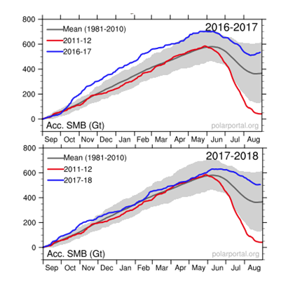
SMB through 2017-18 (top) and 2018-19 (bottom) shown as blue lines. Grey lines show the 1981-2010 average and red shows the record low of 2011-12. Credit: DMI Polar Portal.
Snowfall over the 2017-18 winter was close to the long-term average and although there were heavy snowfalls – especially in the east of Greenland – there were no record storms as in the previous winter, when we saw the arrival of former tropical hurricanes Matthew and Nicole in October 2016.
The maps below show the gains (blue shading) and losses (red) in ice mass by August for 2017 (left) and 2018 (right). The eastern part of Greenland has had above average SMB in both seasons while the western part has seen considerable losses.
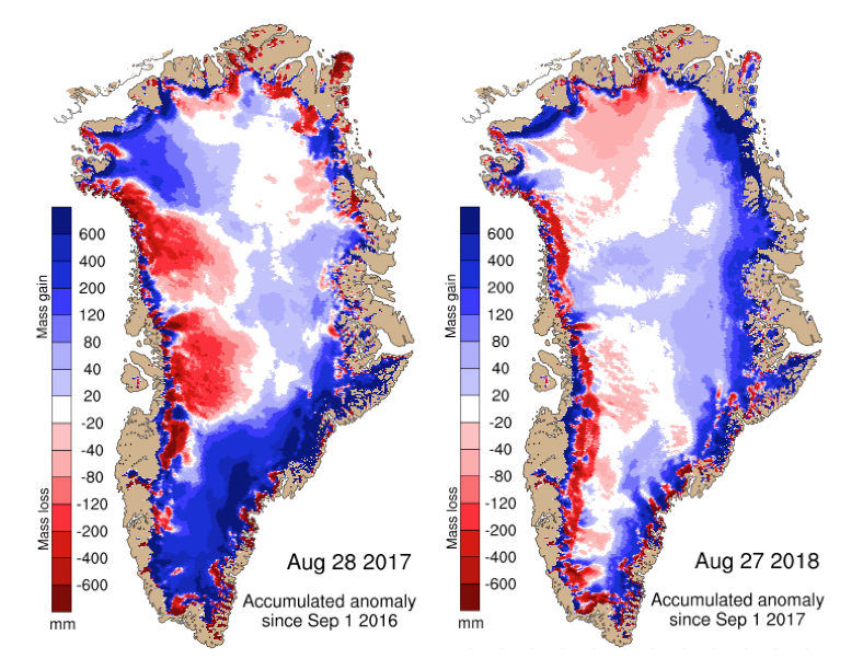
Maps show the difference between the annual SMB in 2017 (left) and 2018 (right) compared with the 1981-2010 period (in mm of ice melt). Blue shows more ice gain than average and red shows more ice loss than average. Credit: DMI Polar Portal.
The melt season started as normal in May, but it was relatively cold month – the Summit Station at the very top of Greenland even set a new record low for the month when it dropped to -46.3C on 9 May. In addition, late spring snowfall in early June restricted melting and the “ablation” season – when ice melts and runs off the ice sheet into the ocean – did not really get going until the last week in June.
Further fresh snow over much of southern Greenland in early July again replenished the snow at the surface and reduced melt rates. Fresh snow not only indicates cold weather, it also reduces melting as it is very bright and reflective compared to darker old snow and bare glacier ice – which often covered in dirt, dust and algae.
Typically, summer melt rates increase as the darker snow and ice is exposed, which absorbs more solar energy, leading to more melting – the so-called “ice-albedo feedback”. This summer, the frequent snow storms replenished the bright white surface on several occasions, holding back the albedo feedback from accelerating melt through the season.
Heatwave and the Atlantic see-saw
While much of the northern hemisphere had a summer of record-breaking heat, Greenland had a rather cool and snowy summer, particularly in the month of June, which ended with a large storm that dumped a large amount of snow on the ice sheet on the last two days of August.
This “see-saw” pattern is a feature of the North Atlantic Oscillation (NAO), a source of variability over the Atlantic Ocean. If it is relatively warm over central and northern Europe, temperatures are below normal in western Greenland – and vice versa.
You can see this below in the maps of air temperature during June. The red shading shows surface warmth over much of Europe, while there is a large patch of blue over Greenland.
This weather pattern persisted for several weeks, which explains why the Greenland ice sheet was colder than usual and had more snow than normal.
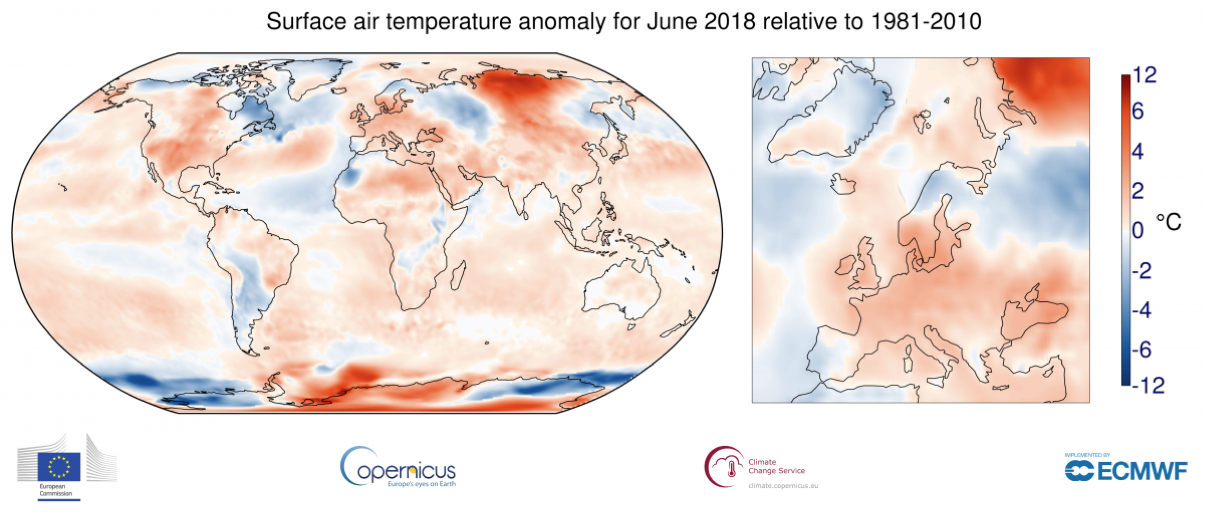
Maps show average temperature for June 2018, relative to 1981-2010 average. Shading indicates warm (red) and cool (blue) areas. Credit: Copernicus Climate Change Service / ECMWF
By the middle of August, the prolonged heat in Europe had finally broken and more normal weather came back to Scandinavia – as the temperature maps (below) for August show.
This was also a period with strong southerly winds in northern Greenland. These “foehn” winds were strong enough to drive sea ice away from the coast of Greenland where it is usually stubbornly fixed. It also coincided with a period of high temperatures, including a new record for high of 17C recorded at Kap Morris Jesup, the northernmost tip of Greenland.
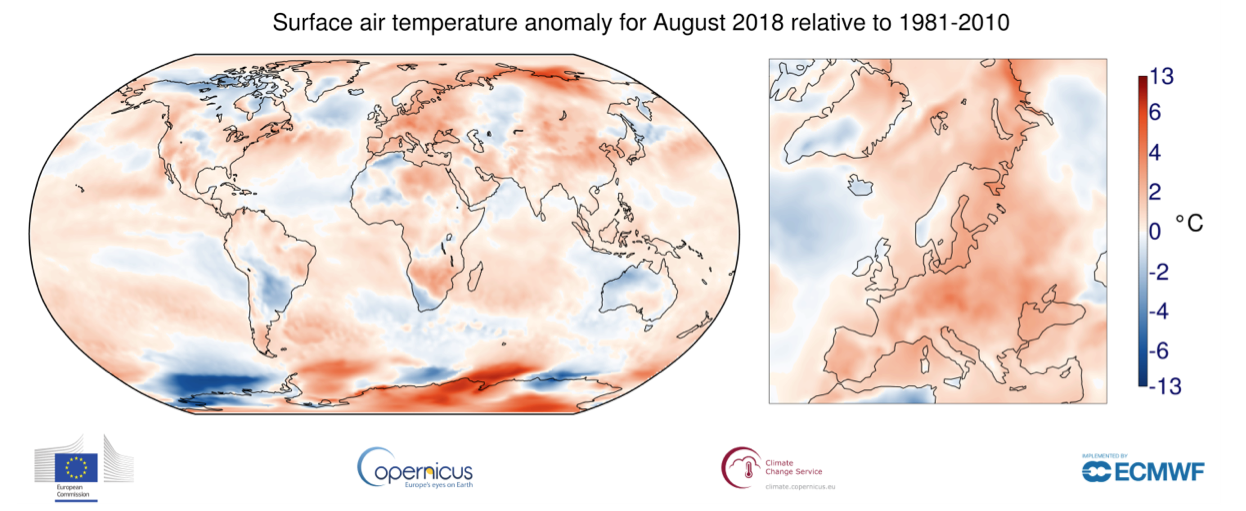
Maps show average temperature for August 2018, relative to 1981-2010 average. Shading indicates warm (red) and cool (blue) areas. Credit: Copernicus Climate Change Service / ECMWF
Total mass balance and looking forward to GRACE-FO
Our analysis shows that the year-to-year variability in SMB can be high and is highly dependent on the weather. But what about the total mass budget – that also accounts for mass loss via calving and melting at the base of the ice sheet? Well there is good news and bad news.
The bad news is that the GRACE satellite that can measure the mass change has not given any reliable data since June 2016. The good news is that the successor, GRACE-FO, launched in May and has already started giving some early observations.
When the data become available we will again be monitoring the total mass balance of Greenland with more confidence – with updates on the Polar Portal.
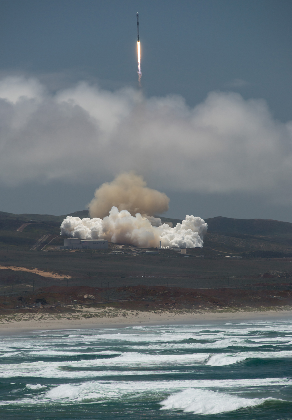
The NASA/German Research Centre for Geosciences GRACE Follow-On spacecraft launches onboard a SpaceX Falcon 9, 22 May 2018, from Vandenberg Air Force Base in California. Credit: NASA/Bill Ingalls