Guest post: How the Greenland ice sheet fared in 2022

The end of the northern-hemisphere summer brings to a close the Greenland ice sheet melt season and with it confirmation that 2022 was the 26th year in a row where Greenland lost ice overall.

While much of Europe and North America sweltered this summer, Greenland was rather wet and cool, with the melt season delayed by snowfall in June. Melting came to a near-end in mid-August and the summer ended with a huge snowfall event dumping almost 20bn tonnes (Gt) of snow onto south-east Greenland. 

Nonetheless, taking into account surface melting, breaking off of icebergs and frictional effects under glaciers, the Greenland ice sheet lost 84Gt of ice over the 12 months from September 2021 to August 2022. 

Greenland last saw an annual net gain of ice in 1996.

In this annual guest post, we discuss the processes of ice sheet melt, glacier calving, weather and climate that explain these losses. This year, we extend our discussion slightly and also look at the unusual warm period in the beginning of September 2022.

(See our previous annual analysis for 2021, 2020, 2019, 2018, 2017, 2016 and 2015.)

Surface melt

As ever with our annual Greenland review, we focus on the 12 months up until the end of August. 

Greenland’s annual cycle sees the ice sheet largely gain snow from September, accumulating ice through autumn, winter and into spring. Then, as the year warms up into late spring, the ice sheet begins to lose more ice through surface melt than it gains from fresh snowfall. This melt season generally continues until the end of August. 

The snow gains and ice losses at the ice sheet’s surface over the past 12 months are the “surface mass balance” (SMB) of the ice sheet. 

Below, we show data from the Polar Portal. The blue line in the upper chart shows the day-to-day SMB. The blue line in the lower chart depicts the accumulated SMB, counted from the beginning of the “mass balance year” on 1 September 2021. In grey, the long-term average and its variability are shown. The red line shows the record low year of 2011-12 for comparison.

The map shows the geographic spread of SMB gains (blue) and losses (red) for 2021-22, compared to the long-term average. 

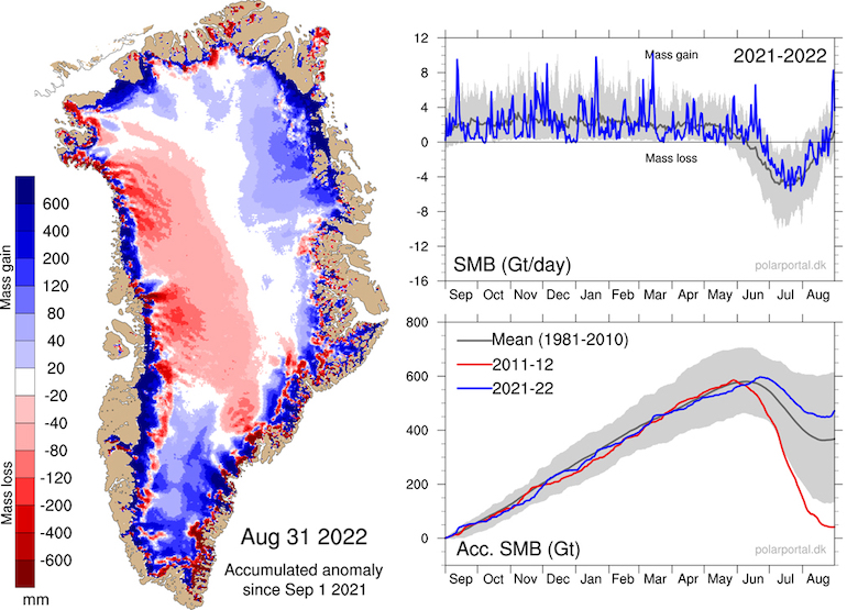
According to our calculations, this year the Greenland ice sheet ended with a total SMB of about 471Gt. This means that 2021-22 ranks the 10th highest for SMB in our dataset that goes back 42 years.

Under current climate conditions, 2021-22 can be considered a relatively favourable year for the ice sheet. Up to the mid-2000s, it would rather have been seen as an average year.

See-saw

Closer inspection of the weather and ice sheet changes through the past 12 months reveal some fascinating events and patterns.

The overall weather pattern during winter resembled the situation of the previous year. Winter snowfall over 2021-22 was close to average, which again is good news for the health of the ice sheet. (Although limited winter snowfall followed by a warm summer – as in 2019 – can lead to considerable ice losses.)

In a similar way to the previous year, the summer was characterised by several large snow events. Snowfall in June delayed the onset of the main part of the melt – or “ablation” – season. Fresh snow is white and reflects sunlight better than the old dark glacier ice underneath. As a result, the onset of melting – which is defined as the first day of three days in a row where the SMB is less than -1Gt – was on 30 June, 17 days later than the median for 1981-2021.

A similar situation took place at the end of the summer, when near record snowfall was dumped onto the south-east of Greenland, adding 20Gt to the surface mass balance.

The reason for these wet – and also cold – spells over the Greenland ice sheet has to do with atmospheric blocking. These high-pressure “blocking” weather systems can have a huge impact on weather extremes. 

For example, in the summer of 2021, a high-pressure “blocking” weather system stalled over south-western Canada and north-western US, triggering a record-breaking “heat dome”. 

And, this year, blocking over Europe led to record-high temperatures in many countries and the continent’s warmest summer on record. A rapid-attribution study revealed that such a heatwave, with temperature exceeding 40C in the UK, would have been “extremely unlikely” without the underlying influence of human-caused warming. 

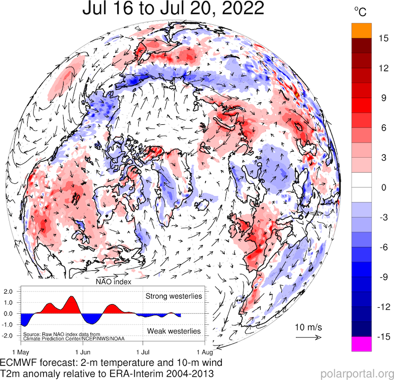
While Europe sizzled, several blocking systems also formed over the western part of Canada and the US, with the jet stream shaped like the capital Greek letter Omega (Ω). With the jet stream diverted far to the north into the Canadian Arctic, troughs of low pressure at the “feet” of the Omega left one over Alaska and the other one over Greenland. This led to the rather cool and wet summer. 

The map below shows the cool summer weather in Greenland (in the centre of the map, shaded mostly blue) in mid-July and the abnormal heat over the western half of North America and, in particular, over Europe (red shading on left-hand and right-hand side, respectively).

Intense melt

Despite the cool start, as the melt season got underway there was a period of very high temperatures at the end of July. This brought intense melt all around the ice sheet that led to very large ice losses over a few days.

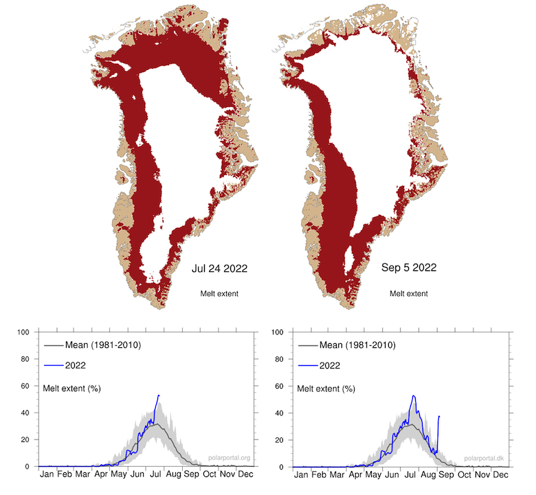
The left-hand map below shows the area of ice melt on 24 July when this summer’s maximum was reached (red shading), and the chart beneath confirms that almost 60% of the ice sheet’s surface was melting on that day. 

The map on the right side shows the large area of melt on 3 September, which is highly unusual for the time of the year. 

This period saw temperature anomalies larger than 20C over western Greenland and a large increase of the surface mass balance, mainly due to rainfall. As this rain percolates into the snowpack and refreezes, it might later on impede further percolation and, thus, increase the runoff during the next warm period.

Components of the mass balance

Following research published late last year, it is possible to distinguish between the components of the “total” mass balance (TMB) as follows:

TMB = SMB + MMB + BMB

Here, MMB is the “marine” mass balance, consisting of the breaking off – or “calving” – of icebergs and the melting of the front of glaciers where they meet the warm sea water. BMB is the “basal” mass balance, which refers to ice losses from the base of the ice sheet. This makes a small, but non-zero, contribution to the TMB and mainly consists of frictional effects and the ground heat flux.

The components of the total mass balance going back to 1987 are shown in the figure below. Here, the SMB is shown in blue, the MMB in green, the BMB in yellow and the TMB in red. 

For the past year, the TMB clocked in at a loss of 84Gt of ice. This means that 2021-22 was the 26th year in a row where the Greenland ice sheet has lost mass overall. Greenland last saw an annual net gain of ice in 1996.

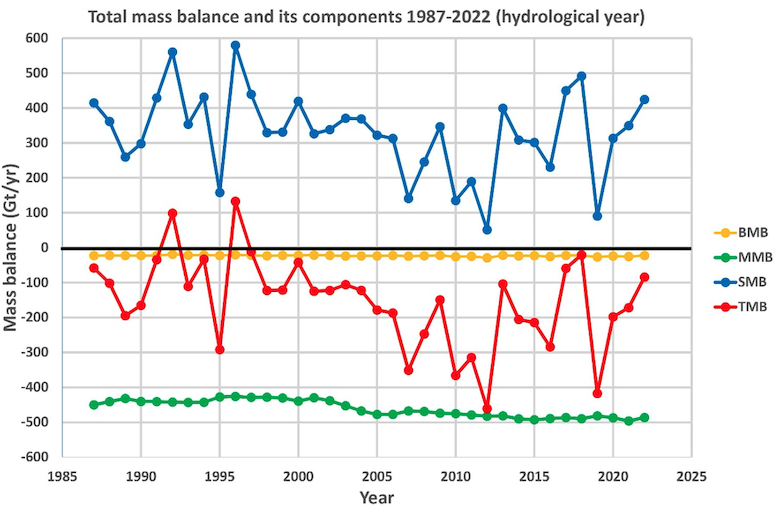
The chart highlights that the only way for the ice sheet to gain ice is via the SMB – that is, through snowfall. The other components, MMB and BMB, are always negative, so the surplus of snowfall over runoff and the two other components needs to be large enough.

By means of the GRACE satellites, we can estimate the TMB independently. The distance of these twin satellites changes slightly due to tiny gravity differences caused by mass changes. However, expressing these distance differences as mass changes is not straightforward, which is the reason why GRACE data always is a lagging few months behind.

Furthermore, using satellites, we can measure the speed at which ice flows through control points on the ice sheet where we know the thickness and shape of the ice. Thus, we can estimate MMB, the amount of ice being lost by the process of calving and submarine melting. This data is openly available, allowing us to monitor the whole ice sheet budget. 

The map and graph below show the gain (blue) and loss (red) in the mass of ice from the GRACE data, relative to April 2002. The difference in these mass changes over a glaciological year (September to August) is the TMB of the Greenland ice sheet for that particular year.

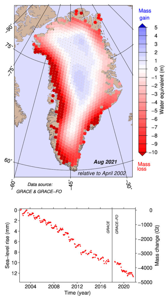
The map shows that most of the loss of ice occurs along the edge of the ice sheet, where independent observations also indicate that the ice is thinning. High up in central Greenland, there is a small increase in the mass of the ice. Independent measurements suggest that this is due to a small increase in snowfall.

The graph illustrates the month-by-month development in changes of mass, relative to April 2002. The left axis on the graph shows how this ice mass loss corresponds to sea level rise contribution, where 100Gt corresponds to 0.28mm global sea level rise.

From 1 April 2002 to 31 August 2021, the period common to both datasets, the Greenland ice sheet has lost approximately 4,500Gt of ice. This is equivalent to 13mm of global average sea level rise. For context, a recent study estimated that climate change to date means that Greenland is already committed to “at least 274mm” of future sea level rise.