Guest post: The role ‘emulator’ models play in climate change projections

The most state-of-the-art tool available to climate scientists is, perhaps, the Earth System Model (ESM). These climate models simulate the flow of energy, moisture and chemicals through the atmosphere, ocean and land surface in unprecedented detail.

However, they need considerable time and expense to run – requiring powerful supercomputers and teams of climate scientists and software engineers to produce the models and analyse the results. 

To speed things up, scientists have the option of using a type of simpler model – known as “emulators” – to provide projections. While ESMs can have millions of lines of computer code, an emulator may have just hundreds or thousands.

While some emulators effectively act as simple climate models – taking future emissions scenarios and projecting greenhouse gas concentrations and global temperature change – others are used for more specific purposes. These models might be used for determining sea level rise from melting ice sheets and glaciers, or translating global temperature rise into regional climate change. 

In this article, I unpack what emulators are, how they are used in climate science, and the role they play in the sixth assessment report (AR6) of the Intergovernmental Panel on Climate Change (IPCC).

Long history

Emulators have been around nearly as long as more sophisticated climate models. US climate scientist Dr James Hansen and his colleagues proposed a simple climate model back in 1981 that was based on concentrations of atmospheric CO2 and the activity of volcanoes and the sun. It has since been shown to have reproduced observed warming well. 

The IPCC has used emulators throughout its history. In its first four assessment reports, the Working Group 1 (WG1) part – which focuses on the underlying climate science – used emulators to project future warming under a number of emissions scenarios and supplement knowledge from the climate models available at the time. This period coincided with the development of the emulator “MAGICC” (Model for the Assessment of Greenhouse gas-Induced Climate Change), on which the majority of the IPCC projections were based.

In the fifth assessment report (AR5), ESMs began to dominate future climate projections, not least due to the coordinated Coupled Model Intercomparison Project (CMIP5), which provided 30 or so ESM projections out to 2100 under different emissions scenarios.

For the recently released AR6 WG1 report, emulators have returned to a more prominent role, being used once again to support, extend and constrain climate projections from ESMs. This is despite an updated set of ESM runs being available from the latest model intercomparison project (CMIP6). 

One challenge in using raw CMIP6 results from ESMs is the number of models that lie outside the AR6 assessed “very likely” range of equilibrium climate sensitivity (ECS) of between 2C and 5C – particularly at the high end. ECS is a measure of how much global average temperatures will eventually rise after atmospheric CO2 reaches double the levels seen before the Industrial Revolution.

Coupled with high rates of simulated near-term warming, this leads to very high levels of projected future warming in several CMIP6 models. Using emulators that have been calibrated to the AR6 assessed range of ECS, in combination with observationally constrained results from CMIP6, brings down the high end-of-century projected future warming by some CMIP6 models.

This is an example of a feature common to all emulators – they have a number of parameters, such as ECS, that can be varied to change the behaviour of the model. 

A simple climate model emulator may contain up to 100 or so different parameters that control different aspects of the climate system, such as the warming and cooling impact of air pollution, how heat diffuses in the ocean, and the response of land and ocean carbon sinks to global warming.

By simultaneously varying parameters, emulators can be “tuned” to replicate the behaviour of ESMs. This is performed using the vast array of ESM output data available from the CMIP6 archive. Again, using the simple climate model example, each component of the Earth system can be tuned using a different experiment from CMIP6. 

For example, we know that the airborne fraction of CO2 – the proportion of CO2 emitted that remains in the atmosphere following emission – depends on the strength of land and ocean carbon sinks, which in turn are dependent on temperature and total carbon stored in those sinks. We might make an educated guess at the functional form of this relationship, and then fit this relationship to ESM results from dedicated model experiments. 

Validating against observations

Unlike ESMs, emulators are very quick to run and can produce a climate projection in a fraction of a second on a desktop computer. This means that emulators can be run hundreds, thousands or even millions of times for a single emissions scenario with different parameter values. This is important in order to span the range of uncertainty around future climate projections. 

In each run, the parameters will be varied – usually sampled at random within predefined distributions – to produce a different climate projection. The parameter values may be sampled from distributions that are based on the CMIP6 model tunings, or from other prior knowledge, such as a very likely range for ECS.

Not all parameter combinations will produce realistic climate projections. One indicator of “realism” is whether an emulator can reproduce a good representation of the historically observed climate change. 

As we can run very large sets of emulator projections, we can throw out simulations that do not correspond well to historical climate change. We can compare model output with, for example, observed global average temperature rise, the change in ocean heat uptake, and whether an emulator’s CO2 concentrations match observed values. 

Knowing observations are not perfect themselves, we can build in the observational uncertainty around these best estimate values, too. This results in a much smaller, constrained set of projections than we started with, but one in which we can have more confidence.

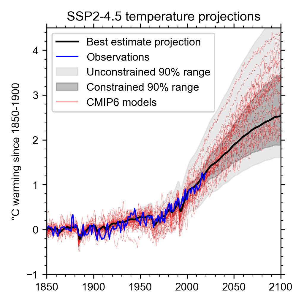
You can see this in the figure below, which shows how global warming in CMIP6 models (red lines) compare to historical temperature observations (blue). Using our emulator that is calibrated to CMIP6 results, we can produce a range of projections (light grey). However, when we introduce our observational constraints, we substantially narrow the range of uncertainty in future projections (dark grey) by eliminating some of the more implausible projections, producing a best estimate future projection (black) that closely follows the observed warming. This method corrects for some of the systematic biases in CMIP6 models, for example a tendency to underpredict the warming in the late 20th Century.

Multiple scenarios

One of the many strengths of emulators is that they can be used to run climate scenarios not analysed by ESMs. The Shared Socioeconomic Pathways (SSPs) developed for running in ESMs for CMIP6 only contain nine future scenarios – five of which are designated as “headline” scenarios. The number of scenarios are necessarily limited due to ESM run time and availability of supercomputers in modelling centres around the world. 

Additionally, many relevant physical science questions depend on running simulations that were not performed in CMIP6 and, as such, are best suited to emulators. 

One prominent example is the attribution of present-day warming to emissions of different gases and aerosols, which you can see in the chart below. The bars indicate emissions that have an overall warming (red) or cooling (blue) effect, with the total human-caused impact shown in grey.

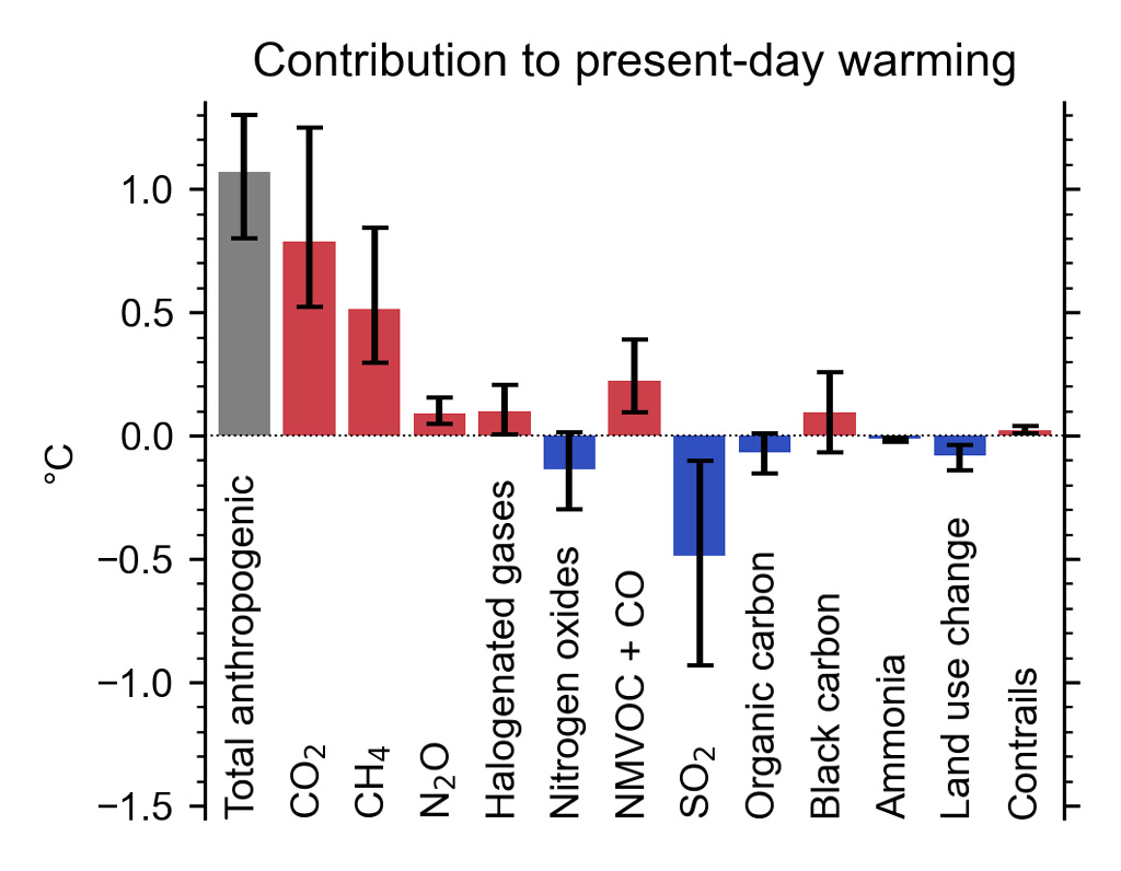
Using an emulator, the differences in radiative forcing are calculated with and without each type of emission present, and these forcings are then converted to a temperature contribution. 

Being able to run a large number of simulations means that the uncertainty in the temperature response to each forcing can be estimated – and using a constrained set of parameters means that the results reported are fully consistent with observed overall warming. 

Other uses of emulators in AR6 include estimating climate change to periods not well-covered by the model scenarios (pre-1850 or post-2100) or for determining climate phenomena absent in most ESMs – such as sea-level contribution from land ice and glacier melt, or methane release from permafrost melt. 

Together, these reasons lead to an extensive use of emulators in the WG1 report, which is summarised in the table below.

Location in AR6	Use of emulators	Why emulators are used
Summary for Policymakers	Determining the contribution to present-day (SPM Fig. 2) and future (SPM Fig. 4) warming from individual emissions or radiative forcings	No CMIP6 model results available Reported results are fully consistent with AR6 assessed ranges of climate sensitivity and present-day and future warming
Chapter 1	Estimating anthropogenic temperature contribution from 1750 to 1850	No pre-1850 anthropogenic experiments available in CMIP6
Chapter 3	Determining the contribution to present-day warming from individual forcings	Reported results are fully consistent with AR6 assessed ranges of climate sensitivity and present-day and future warming
Chapter 4	Determining future warming estimates from five SSPs	Some CMIP6 models show implausibly high near-term warming rates and high climate sensitivity, leading to very high warming projections from the unconstrained CMIP6 model archive Assessed future warming is fully consistent with AR6-assessed ECS and TCR
Chapter 4	Demonstrating the difference in radiative forcing and temperature projections between RCP and SSP scenarios	Very few ESMs ran both RCP and SSP projections in the same model, making direct comparison impossible Difficulty of diagnosing radiative forcing from coupled ESMs
Chapter 4	Extending temperature projections beyond 2100	Only a handful of CMIP6 models ran projections beyond 2100 and those that did were biased towards high sensitivity models
Chapter 5	Estimating non-CO2 contributions to the remaining carbon budget	No equivalent CMIP6 experiments
Chapter 6	Determining the contribution to present-day warming from individual emissions	No CMIP6 model results available
Chapter 7	Estimating processed-based TCR from a processed-based ECS	Specific emulator parameter set required that does not match any particular CMIP6 model
Chapter 7	Greenhouse gas metrics of Global Warming Potential and Global Temperature Potential	Over 400 greenhouse gases assessed, only a small subset are modelled in ESM radiative transfer codes Almost impossible to perform in ESM as small radiative forcings and temperature responses in the GWP and GTP definition would be dominated by internal variability
Chapter 9	Global mean sea-level projections	Some contributions to sea-level rise such as land ice sheet and glacier loss are not modelled by ESMs Only a handful of CMIP6 models ran projections beyond 2100
Chapter 11	Regional climate change at different global warming levels	Reported results are fully consistent with AR6 assessed ranges of future warming

Summary of emulator use in the IPCC WG1 AR6, Adapted and extended from the IPCC AR6 WG1 (2021) Cross-Chapter Box 7.1 by Chris Smith.

Coordination

The ability for emulators to quickly run scenarios that are not used by ESMs is vitally important for the Working Group 3 (WG3) contribution to AR6 – which focuses on climate change mitigation – expected in early 2022.

WG3 has long used emulators to determine the global average warming response to future emission pathways derived by Integrated Assessment Models (IAMs). The sheer number of IAM scenarios submitted for analysis by the IPCC – more than 1,000 in AR5 and more than 400 in the IPCC’s special report on 1.5C – necessitates the use of efficient models to make climate projections. This number of simulations would not be feasible in ESMs, particularly if the full uncertainty range in future projections is desired.

One major advance in AR6 is the closer collaboration between WG1 in developing and testing emulators and WG3 in assessing IAM pathways. The WG1 report considers four climate model emulators: 

• MAGICC (developed at University of Melbourne, Australia);
• FaIR (University of Leeds/University of Oxford, UK);
• OSCAR (IIASA, Austria); and 
• CICERO-SCM (CICERO, Norway). 

These four are by no means the only ones available, but were considered by the IPCC as the ones with an ability to convert a wide range of different human-caused emissions first to greenhouse gas concentrations, then radiative forcing and finally global average temperature.

In WG1, the MAGICC, FaIR, CICERO and OSCAR emulators were rigorously tested and compared to multiple assessed constraints contained within the report – such as ECS, warming since pre-industrial and ocean heat content change. Three of the four emulators were deemed suitable for delivery to WG3, where each will be used to run potentially thousands of IAM emissions scenarios. This ensures that the emulators used by WG3 are fully consistent with the most up-to-date climate science. 

It is very likely that coordination between the physical climate and socioeconomic aspects of climate science will continue to develop. An emerging research area is the interaction between climate change and the energy system. 

For example, existing emissions scenarios from IAMs do not account for human-system feedbacks – such as the fact that warmer summers projected in a changing climate will increase demand for air conditioning, which increases energy demand and therefore increases emissions if the grid is not zero-carbon, leading to further warming. Emulators will play a key role in translating climate knowledge efficiently between ESMs and IAMs.

Emulators may have gained prominence in AR6, but that is not to say that they are a replacement for ESMs. There are some things that only ESMs can do – for example, they are necessary for a deeper dive into the statistics of climate change, particularly the changes in weather extremes that are most devastating for human and natural ecosystems.

In general, emulators are not developed by the same groups who work on ESMs. This brings objectivity and independence to the simultaneous usage of the two levels of model complexity. 

As climate models continue to increase in resolution, they can begin to explicitly resolve localised processes – such as convection, the behaviour of clouds and circular ocean currents called “eddies” – and lead us to greater insight of these individual processes, their feedbacks and interactions, and how they might be affected by climate change. 

However, with the ongoing development of cleverly designed emulators, we can use the benefits of this cutting-edge science to create projections from models that are cheap and easy to run. This combination of the simple with the complex is a real strength in the IPCC’s AR6.