In the first article of a week-long series focused on climate modelling, Carbon Brief explains in detail how scientists use computers to understand our changing climate…
The use of computer models runs right through the heart of climate science.
From helping scientists unravel cycles of ice ages hundreds of thousands of years ago to making projections for this century or the next, models are an essential tool for understanding the Earth’s climate.
But what is a climate model? What does it look like? What does it actually do? These are all questions that anyone outside the world of climate science might reasonably ask.
Carbon Brief has spoken to a range of climate scientists in order to answer these questions and more. What follows is an in-depth Q&A on climate models and how scientists use them. You can use the links below to navigate to a specific question.
- What is a climate model?
- What are the different types of climate models?
- What are the inputs and outputs for of a climate model?
- What types of experiments do scientists run on climate models?
- Who does climate modelling around the world?
- What is CMIP?
- How do scientists validate climate models? How do they check them?
- How are climate models “parameterised” and tuned?
- What is bias correction?
- How accurate are climate model projections of temperature?
- What are the main limitations in climate modelling at the moment?
- What is the process for improving models?
- How do scientists produce climate model information for specific regions?
What is a climate model?
A global climate model typically contains enough computer code to fill 18,000 pages of printed text; it will have taken hundreds of scientists many years to build and improve; and it can require a supercomputer the size of a tennis court to run.
The models themselves come in different forms – from those that just cover one particular region of the world or part of the climate system, to those that simulate the atmosphere, oceans, ice and land for the whole planet.
The output from these models drives forward climate science, helping scientists understand how human activity is affecting the Earth’s climate. These advances have underpinned climate policy decisions on national and international scales for the past five decades.
In many ways, climate modelling is just an extension of weather forecasting, but focusing on changes over decades rather than hours. In fact, the UK’s Met Office Hadley Centre uses the same “Unified Model” as the basis for both tasks.
The vast computing power required for simulating the weather and climate means today’s models are run using massive supercomputers.
The Met Office Hadley Centre’s three new Cray XC40 supercomputers, for example, are together capable of 14,000 trillion calculations a second. The timelapse video below shows the third of these supercomputers being installed in 2017.
Fundamental physical principles
So, what exactly goes into a climate model? At their most basic level, climate models use equations to represent the processes and interactions that drive the Earth’s climate. These cover the atmosphere, oceans, land and ice-covered regions of the planet.
The models are based on the same laws and equations that underpin scientists’ understanding of the physical, chemical and biological mechanisms going on in the Earth system.
For example, scientists want climate models to abide by fundamental physical principles, such as the first law of thermodynamics (also known as the law of conservation of energy), which states that in a closed system, energy cannot be lost or created, only changed from one form to another.
Another is the Stefan-Boltzmann Law, from which scientists have shown that the natural greenhouse effect keeps the Earth’s surface around 33C warmer than it would be without one.
Then there are the equations that describe the dynamics of what goes on in the climate system, such as the Clausius-Clapeyron equation, which characterises the relationship between the temperature of the air and its maximum water vapour pressure.
The most important of these are the Navier-Stokes equations of fluid motion, which capture the speed, pressure, temperature and density of the gases in the atmosphere and the water in the ocean.
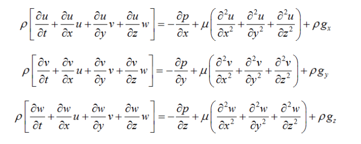
The Navier-Stokes equations for “incompressible” flow in three dimensions (x, y and z). (Although the air in our atmosphere is technically compressible, it is relatively slow-moving and is, therefore, treated as incompressible in order to simplify the equations.). Note: this set of equations is simpler than the ones a climate model will use because they need to calculate flows across a rotating sphere.
However, this set of partial differential equations is so complex that there is no known exact solution to them (except in a few simple cases). It remains one of the great mathematical challenges (and there is a one million dollar prize awaiting whoever manages to prove a solution always exists). Instead, these equations are solved “numerically” in the model, which means they are approximated.
Scientists translate each of these physical principles into equations that make up line after line of computer code – often running to more than a million lines for a global climate model.
The code in global climate models is typically written in the programming language Fortran. Developed by IBM in the 1950s, Fortran was the first “high-level” programming language. This means that rather than being written in a machine language – typically a stream of numbers – the code is written much like a human language.
You can see this in the example below, which shows a small section of code from one of the Met Office Hadley Centre models. The code contains commands such as “IF”, “THEN” and “DO”. When the model is run, it is first translated (automatically) into machine code that the computer understands.
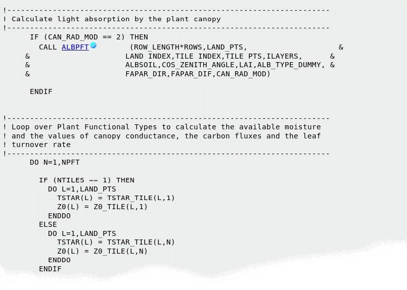
A section of code from HadGEM2-ES (as used for CMIP5) in Fortran programming language. The code is from within the plant physiology section that starts to look at how the different vegetation types absorb light and moisture. Credit: Dr Chris Jones, Met Office Hadley Centre
There are now many other programming languages available to climate scientists, such as C, Python, R, Matlab and IDL. However, the last four of these are applications that are themselves written in a more fundamental language (such as Fortran) and, therefore, are relatively slow to run. Fortran and C are generally used today for running a global model quickly on a supercomputer.
Spatial resolution
Throughout the code in a climate model are equations that govern the underlying physics of the climate system, from how sea ice forms and melts on Arctic waters to the exchange of gases and moisture between the land surface and the air above it.
The figure below shows how more and more climate processes have been incorporated into global models over the decades, from the mid-1970s through to the fourth assessment report (“AR4”) of the Intergovernmental Panel of Climate Change (IPCC), published in 2007.
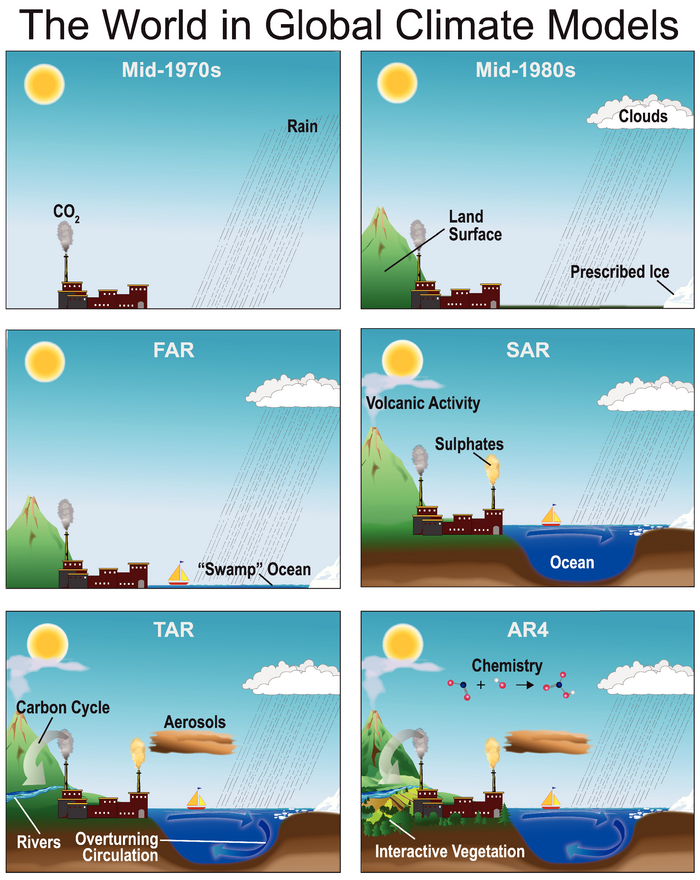
Illustration of the processes added to global climate models over the decades, from the mid-1970s, through the first four IPCC assessment reports: first (“FAR”) published in 1990, second (“SAR”) in 1995, third (“TAR”) in 2001 and fourth (“AR4”) in 2007. (Note, there is also a fifth report, which was completed in 2014). Source: IPCC AR4, Fig 1.2
So, how does a model go about calculating all these equations?
Because of the complexity of the climate system and limitation of computing power, a model cannot possibly calculate all of these processes for every cubic metre of the climate system. Instead, a climate model divides up the Earth into a series of boxes or “grid cells”. A global model can have dozens of layers across the height and depth of the atmosphere and oceans.
The image below shows a 3D representation of what this looks like. The model then calculates the state of the climate system in each cell – factoring in temperature, air pressure, humidity and wind speed.
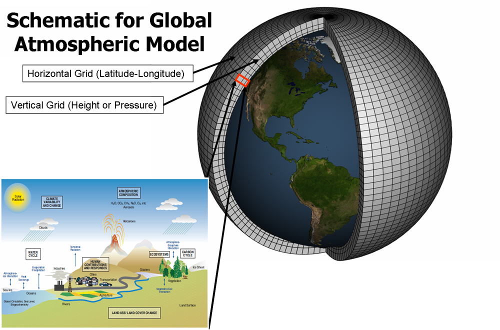
Illustration of grid cells used by climate models and the climatic processes that the model will calculate for each cell (bottom corner). Source: NOAA GFDL
For processes that happen on scales that are smaller than the grid cell, such as convection, the model uses “parameterisations” to fill in these gaps. These are essentially approximations that simplify each process and allow them to be included in the model. (Parameterisation is covered in the question on model tuning below.)
The size of the grid cells in a model is known as its “spatial resolution”. A relatively-coarse global climate model typically has grid cells that are around 100km in longitude and latitude in the mid-latitudes. Because the Earth is a sphere, the cells for a grid based on longitude and latitude are larger at the equator and smaller at the poles. However, it is increasingly common for scientists to use alternative gridding techniques – such as cubed-sphere and icosahedral – which don’t have this problem.
A high-resolution model will have more, smaller boxes. The higher the resolution, the more specific climate information a model can produce for a particular region – but this comes at a cost of taking longer to run because the model has more calculations to make.
The figure below shows how the spatial resolution of models improved between the first and fourth IPCC assessment reports. You can see how the detail in the topography of the land surface emerges as the resolution is improved.
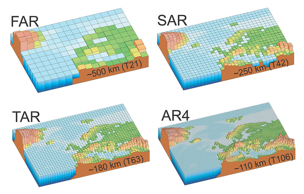
Increasing spatial resolution of climate models used through the first four IPCC assessment reports: first (“FAR”) published in 1990, second (“SAR”) in 1995, third (“TAR”) in 2001 and fourth (“AR4”) in 2007. (Note, there is also a fifth report, which was completed in 2014). Source: IPCC AR4, Fig 1.2
In general, increasing the spatial resolution of a model by a factor of two will require around 10 times the computing power to run in the same amount of time.
Time step
A similar compromise has to be made for the “time step” of how often a model calculates the state of the climate system. In the real world, time is continuous, yet a model needs to chop time up into bite-sized chunks to make the calculations manageable.
Each climate model does this in some way, but the most common approach is the “leapfrogging method”, explains Prof Paul Williams, professor of atmospheric science at the University of Reading, in a book chapter on this very topic:
“The role of the leapfrog in models is to march the weather forward in time, to allow predictions about the future to be made. In the same way that a child in the playground leapfrogs over another child to get from behind to in front, the model leapfrogs over the present to get from the past to the future.”
In other words, the model takes the climate information it has from the previous and present time steps to extrapolate forwards to the next one, and so on through time.
As with the size of grid cells, a smaller time step means the model can produce more detailed climate information. But it also means the model has more calculations to do in every run.
For example, calculating the state of the climate system for every minute of an entire century would require over 50m calculations for every grid cell – whereas only calculating it for each day would take 36,500. That’s quite a range – so how do scientists decide what time step to use?
The answer comes down to finding a balance, Williams tells Carbon Brief:
“Mathematically speaking, the correct approach would be to keep decreasing the time step until the simulations are converged and the results stop changing. However, we normally lack the computational resources to run the models with a time step this small. Therefore, we are forced to tolerate a larger time step than we would ideally like.”
For the atmosphere component of climate models, a time step of around 30 minutes “seems to be a reasonable compromise” between accuracy and computer processing time, says Williams:
“Any smaller and the improved accuracy would not be sufficient to justify the extra computational burden. Any larger and the model would run very quickly, but the simulation quality would be poor.”
Bringing all these pieces together, a climate model can produce a representation of the whole climate system at 30-minute intervals over many decades or even centuries.
As Dr Gavin Schmidt, director of the NASA Goddard Institute for Space Studies, describes in his TED talk in 2014, the interactions of small-scale processes in a model mean it creates a simulation of our climate – everything from the evaporation of moisture from the Earth’s surface and formation of clouds, to where the wind carries them and where the rain eventually falls.
Schmidt calls these “emergent properties” in his talk – features of the climate that aren’t specifically coded in the model, but are simulated by the model as a result of all the individual processes that are built in.
It is akin to the manager of a football team. He or she picks the team, chooses the formation and settles on the tactics, but once the team is out on the pitch, the manager cannot dictate if and when the team scores or concedes a goal. In a climate model, scientists set the ground rules based on the physics of the Earth system, but it is the model itself that creates the storms, droughts and sea ice.
So to summarise: scientists put the fundamental physical equations of the Earth’s climate into a computer model, which is then able to reproduce – among many other things – the circulation of the oceans, the annual cycle of the seasons, and the flows of carbon between the land surface and the atmosphere.
You can watch the whole of Schmidt’s talk below.
While the above broadly explains what a climate model is, there are many different types. Read on to the question below to explore these in more detail.
What are the different types of climate models?
The earliest and most basic numerical climate models are Energy Balance Models (EBMs). EBMs do not simulate the climate, but instead consider the balance between the energy entering the Earth’s atmosphere from the sun and the heat released back out to space. The only climate variable they calculate is surface temperature. The simplest EBMs only require a few lines of code and can be run in a spreadsheet.
Many of these models are “zero-dimensional”, meaning they treat the Earth as a whole; essentially, as a single point. Others are 1D, such as those that also factor in the transfer of energy across different latitudes of the Earth’s surface (which is predominantly from the equator to the poles).
A step along from EBMs are Radiative Convective Models, which simulate the transfer of energy through the height of the atmosphere – for example, by convection as warm air rises. Radiative Convective Models can calculate the temperature and humidity of different layers of the atmosphere. These models are typically 1D – only considering energy transport up through the atmosphere – but they can also be 2D.
The next level up are General Circulation Models (GCMs), also called Global Climate Models, which simulate the physics of the climate itself. This means they capture the flows of air and water in the atmosphere and/or the oceans, as well as the transfer of heat.
Early GCMs only simulated one aspect of the Earth system – such as in “atmosphere-only” or “ocean-only” models – but they did this in three dimensions, incorporating many kilometres of height in the atmosphere or depth of the oceans in dozens of model layers.
More sophisticated “coupled” models have brought these different aspects together, linking together multiple models to provide a comprehensive representation of the climate system. Coupled atmosphere-ocean general circulation models (or “AOGCMs”) can simulate, for example, the exchange of heat and freshwater between the land and ocean surface and the air above.
The infographic below shows how modellers have gradually incorporated individual model components into global coupled models over recent decades.
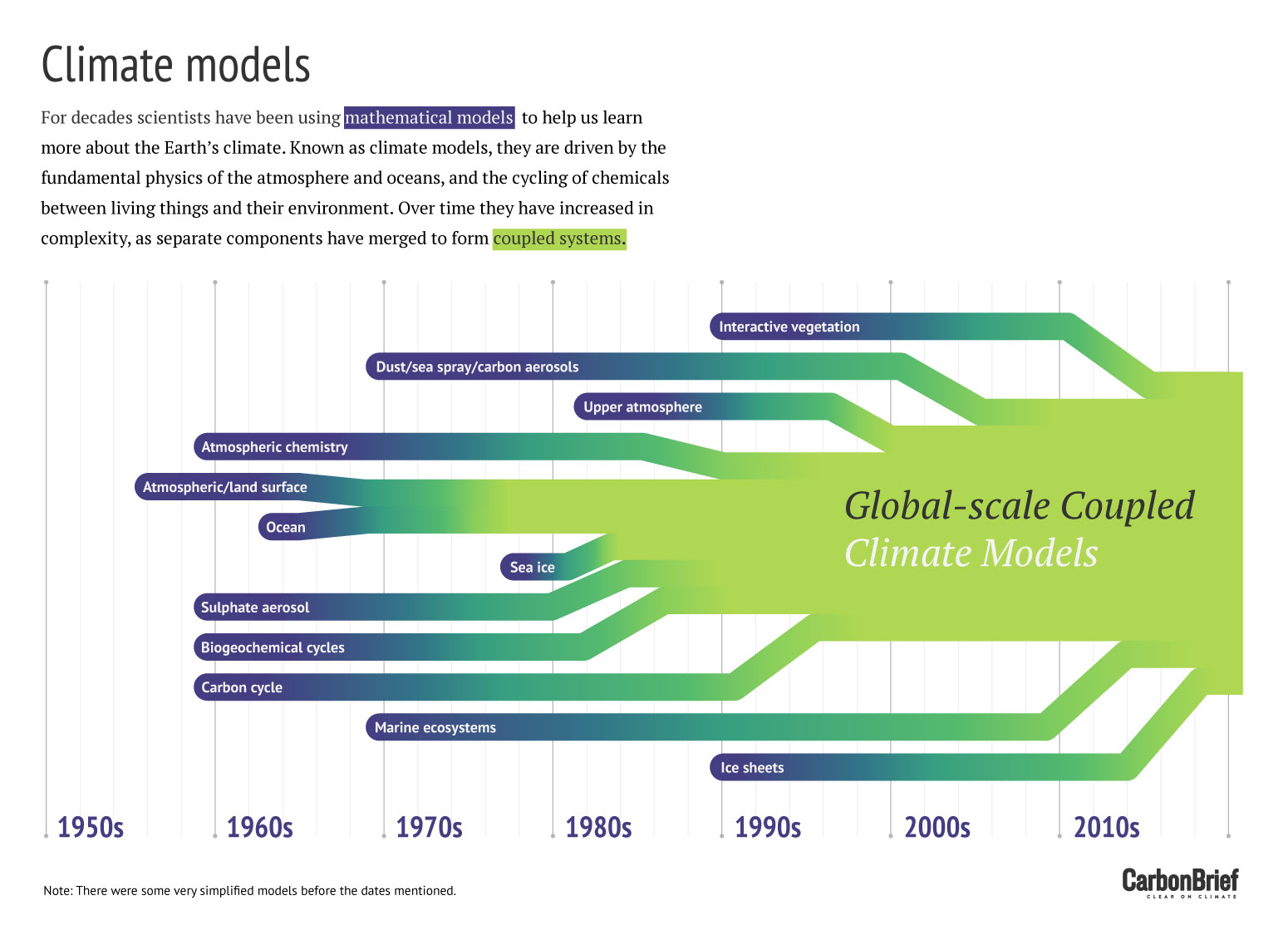
Graphic by Rosamund Pearce; based on the work of Dr Gavin Schmidt.
Over time, scientists have gradually added in other aspects of the Earth system to GCMs. These would have once been simulated in standalone models, such as land hydrology, sea ice and land ice.
The most recent subset of GCMs now incorporate biogeochemical cycles – the transfer of chemicals between living things and their environment – and how they interact with the climate system. These “Earth System Models” (ESMs) can simulate the carbon cycle, nitrogen cycle, atmospheric chemistry, ocean ecology and changes in vegetation and land use, which all affect how the climate responds to human-caused greenhouse gas emissions. They have vegetation that responds to temperature and rainfall and, in turn, changes uptake and release of carbon and other greenhouse gases to the atmosphere.
Prof Pete Smith, professor of soils & global change at the University of Aberdeen describes ESMs as “pimped” versions of GCMs:
“The GCMs were the models that were used maybe in the 1980s. So these were largely put together by the atmospheric physicists, so it’s all to do with energy and mass and water conservation, and it’s all the physics of moving those around. But they had a relatively limited representation of how the atmosphere then interacts with the ocean and the land surface. Whereas an ESM tries to incorporate those land interactions and those ocean interactions, so you could regard an ESM as a ‘pimped’ version of a GCM.”
There are also Regional Climate Models (“RCMs”) which do a similar job as GCMs, but for a limited area of the Earth. Because they cover a smaller area, RCMs can generally be run more quickly and at a higher resolution than GCMs. A model with a high resolution has smaller grid cells and therefore can produce climate information in greater detail for a specific area.
RCMs are one way of “downscaling” global climate information to a local scale. This means taking information provided by a GCM or coarse-scale observations and applying it to a specific area or region. Downscaling is covered in more detail under a later question.
![]()
Finally, a subset of climate modelling involves Integrated Assessment Models (IAMs). These add aspects of society to a simple climate model, simulating how population, economic growth and energy use affect – and interact with – the physical climate.
IAMs produce scenarios of how greenhouse gas emissions may vary in future. Scientists can then run these scenarios through ESMs to generate climate change projections – providing information that can be used to inform climate and energy policies around the world.
In climate research, IAMs are typically used to project future greenhouse gas emissions and the benefits and costs of policy options that could be implemented to tackle them. For example, they are used to estimate the social cost of carbon – the monetary value of the impact, both positive and negative, of every additional tonne of CO2 that is emitted.
What are the inputs and outputs for a climate model?
If the previous section looked at what is inside a climate model, this one focuses on what scientists put into a model and get out the other side.
Climate models are run using data on the factors that drive the climate, and projections about how these might change in the future. Climate model results can run to petabytes of data, including readings every few hours across thousands of variables in space and time, from temperature to clouds to ocean salinity.
Inputs
The main inputs into models are the external factors that change the amount of the sun’s energy that is absorbed by the Earth, or how much is trapped by the atmosphere.
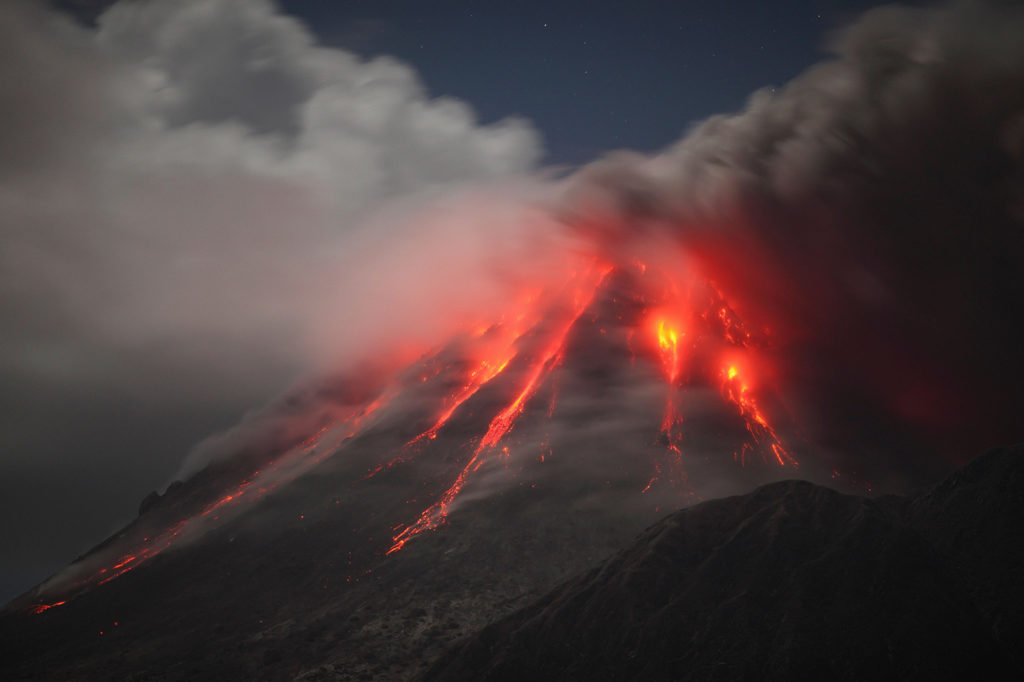
Soufriere Hills eruption, Montserrat Island, Caribbean, 1/2/2010. Credit: Stocktrek Images, Inc./Alamy Stock Photo.
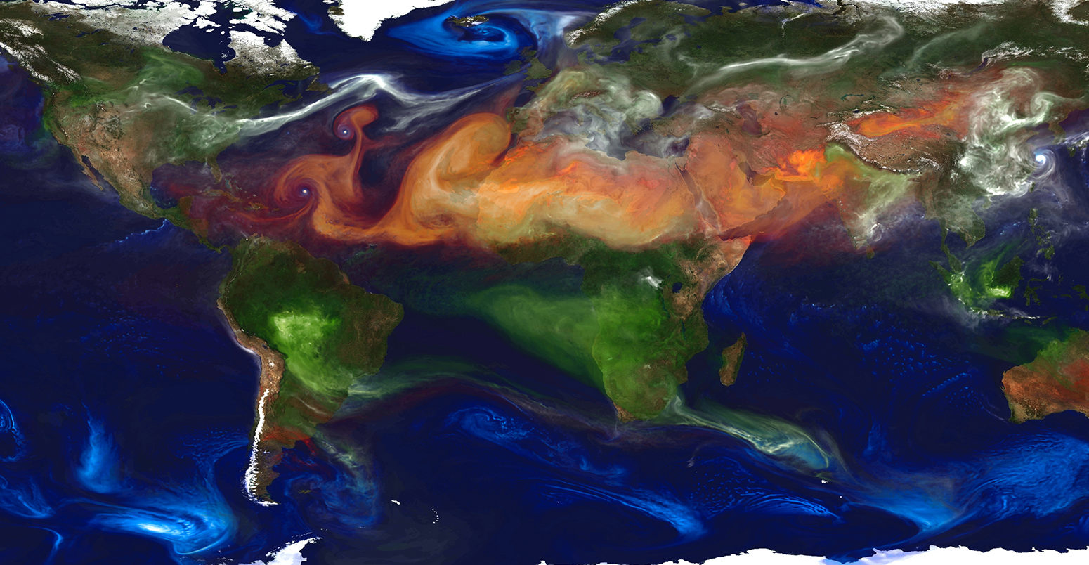
These external factors are called “forcings”. They include changes in the sun’s output, long-lived greenhouse gases – such as CO2, methane (CH4), nitrous oxides (N2O) and halocarbons – as well as tiny particles called aerosols that are emitted when burning fossil fuels, and from forest fires and volcanic eruptions. Aerosols reflect incoming sunlight and influence cloud formation.
Typically, all these individual forcings are run through a model either as a best estimate of past conditions or as part of future “emission scenarios”. These are potential pathways for the concentration of greenhouse gases in the atmosphere, based on how technology, energy and land use change over the centuries ahead.
Today, most model projections use one or more of the “Representative Concentration Pathways” (RCPs), which provide plausible descriptions of the future, based on socio-economic scenarios of how global society grows and develops. You can read more about the different pathways in this earlier Carbon Brief article.
Models also use estimates of past forcings to examine how the climate changed over the past 200, 1,000, or even 20,000 years. Past forcings are estimated using evidence of changes in the Earth’s orbit, historical greenhouse gas concentrations, past volcanic eruptions, changes in sunspot counts, and other records of the distant past.
Then there are climate model “control runs”, where radiative forcing is held constant for hundreds or thousands of years. This allows scientists to compare the modelled climate with and without changes in human or natural forcings, and assess how much “unforced” natural variability occurs.
Outputs
Climate models generate a nearly complete picture of the Earth’s climate, including thousands of different variables across hourly, daily and monthly timeframes.
These outputs include temperatures and humidity of different layers of the atmosphere from the surface to the upper stratosphere, as well as temperatures, salinity and acidity (pH) of the oceans from the surface down to the sea floor.
Models also produce estimates of snowfall, rainfall, snow cover and the extent of glaciers, ice sheets and sea ice. They generate wind speed, strength and direction, as well as climate features, such as the jet stream and ocean currents.
More unusual model outputs include cloud cover and height, along with more technical variables, such as surface upwelling longwave radiation – how much energy is emitted by the surface back up to the atmosphere – or how much sea salt comes off the ocean during evaporation and is accumulated on land.
Climate models also produce an estimate of “climate sensitivity”. That is, they calculate how sensitive the Earth is to increases in greenhouse gas concentrations, taking into account various climate feedbacks, such as water vapour and changes in reflectivity, or “albedo”, of the Earth surface associated with ice loss.
A full list of common outputs from the climate models being run for the next IPCC report are available from the CMIP6 project (the Coupled Model Intercomparison Project 6, or CMIP6; CMIP is explained in more detail, below).
Modellers store petabytes of climate data at locations such as the National Center for Atmospheric Research (NCAR) and often make the data available as netCDF files, which are easy for researchers to analyse.
What types of experiments do scientists run on climate models?
Climate models are used by scientists to answer many different questions, including why the Earth’s climate is changing and how it might change in the future if greenhouse gas emissions continue.
Models can help work out what has caused observed warming in the past, as well as how big a role natural factors play compared to human factors.
Scientists run many different experiments to simulate climates of the past, present and future. They also design tests to look at the performance of specific parts of different climate models. Modellers run experiments on what would happen if, say, we suddenly quadrupled CO2, or if geoengineering approaches were used to cool the climate.
Many different groups run the same experiments on their climate models, producing what is called a model ensemble. These model ensembles allow researchers to examine differences between climate models, as well as better capture the uncertainty in future projections. Experiments that modellers do as part of the Coupled Model Intercomparison Projects (CMIPs) include:
Historical runs
Climate models are run over the historical period, from around 1850 to near-present. They use the best estimate of factors affecting the climate, including CO2, CH4, and N2O concentrations, changes in solar output, aerosols from volcanic eruptions, aerosols from human activity, and land-use changes.
These historical runs are not “fit” to actual observed temperatures or rainfall, but rather emerge from the physics of the model. This means they allow scientists to compare model predictions (“hindcasts”) of the past climate to recorded climate observations. If climate models are able to successfully hindcast past climate variables, such as surface temperature, this gives scientists more confidence in model forecasts of the future
Historical runs are also useful for determining how large a role human activity plays in climate change (called “attribution”). For example, the chart below compares two model variants against the observed climate – with only natural forcings (blue shading) and model runs with both human and natural forcings (pink shading).

Figure from the IPCC’s Fourth Assessment Report (Hegerl et al 2007).
Natural-only runs only include natural factors such as changes in the sun’s output and volcanoes, but they assume greenhouse gases and other human factors remain unchanged at pre-industrial levels. Human-only runs hold natural factors unchanged and only include the effects of human activities, such as increasing atmospheric greenhouse gas concentrations.
By comparing these two scenarios (and a combined “all-factors” run), scientists can assess the relative contributions to observed climate changes from human and natural factors. This helps them to figure out what proportion of modern climate change is due to human activity.
Future warming scenarios
The IPCC’s fifth assessment report focused on four future warming scenarios, known as the Representative Concentration Pathway (RCP) scenarios. These look at how the climate might change from present through to 2100 and beyond.
Many things that drive future emissions, such as population and economic growth, are difficult to predict. Therefore, these scenarios span a wide range of futures, from a business-as-usual world where little or no mitigation actions are taken (RCP6.0 and RCP8.5) to a world in which aggressive mitigation generally limits warming to no more than 2C (RCP2.6). You can read more about the different RCPs here.
These RCP scenarios specify different amounts of radiative forcings. Models use those forcings to examine how the Earth’s system will change under each of the different pathways. The upcoming CMIP6 exercise, associated with the IPCC sixth assessment report, will add four new RCP scenarios to fill in the gaps around the four already in use, including a scenario that meets the 1.5C temperature limit.
Control runs
Control runs are useful to examine how natural variability is expressed in models, in the absence of other changes. They are also used to diagnose “model drift”, where spurious long-term changes occur in the model that are unrelated to either natural variability or changes to external forcing.
If a model is “drifting” it will experience changes beyond the usual year-to-year and decade-to-decade natural variability, even though the factors affecting the climate, such as greenhouse gas concentrations, are unchanged.
Model control runs start the model during a period before modern industrial activity dramatically increased greenhouse gases. They then let the model run for hundreds or thousands of years without changing greenhouse gases, solar activity, or any other external factors that affect the climate. This differs from a natural-only run as both human and natural factors are left unchanged.
Atmospheric model intercomparison project (AMIP) runs
Climate models include the atmosphere, land and ocean. AMIP runs effectively ‘‘turn off’’ everything except the atmosphere, using fixed values for the land and ocean based on observations. For example, AMIP runs use observed sea surface temperatures as an input to the model, allowing the land surface temperature and the temperature of the different layers of the atmosphere to respond.
Normally climate models will have their own internal variability – short-term climate cycles in the oceans such as El Niño and La Niña events – that occur at different times than what happens in the real world. AMIP runs allow modellers to match ocean temperatures to observations, so that internal variability in the models occurs at the same time as in the observations and changes over time in both are easier to compare.
Abrupt 4x CO2 runs
Climate models comparison projects, such as CMIP5, generally request that all models undertake a set of “diagnostic” scenarios to test performance across various criteria.
One of these tests is an “abrupt” increase in CO2 from pre-industrial levels to four times higher – from 280 parts per million (ppm) to 1,120ppm – holding all other factors that influence the climate constant. (For context, current CO2 concentrations are around 400ppm.) This allows scientists to see how quickly the Earth’s temperature responds to changes in CO2 in their model compared to others.
-
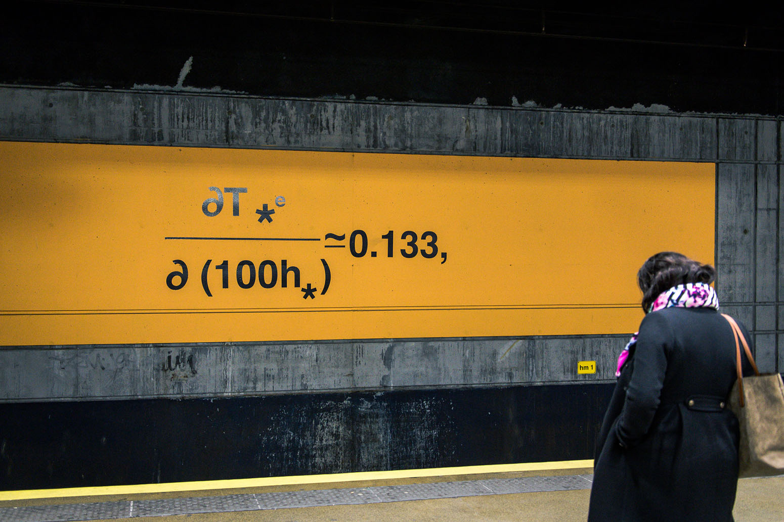
One of 42 panels displayed throughout the Gare du Nord metro station in Paris, honouring Syukuro Manabe and his contributions to climate science, to mark the COP21 UN climate change conference in 2015. The equations were used by Manabe in his seminal climate model in the late 1960s. Credit: NOAA/Rory O'Connor.
-

One of 42 panels displayed throughout the Gare du Nord metro station in Paris, honouring Syukuro Manabe and his contributions to climate science, to mark the COP21 UN climate change conference in 2015. The equations were used by Manabe in his seminal climate model in the late 1960s. Credit: Rosamund Pearce/Carbon Brief.
-

One of 42 panels displayed throughout the Gare du Nord metro station in Paris, honouring Syukuro Manabe and his contributions to climate science, to mark the COP21 UN climate change conference in 2015. The equations were used by Manabe in his seminal climate model in the late 1960s. Credit: NOAA/Rory O'Connor.
1% CO2 runs
Another diagnostic test increases CO2 emissions from pre-industrial levels by 1% per year, until CO2 ultimately quadruples and reaches 1,120ppm. These scenarios also hold all other factors affecting the climate unchanged.
This allows modellers to isolate the effects of gradually increasing CO2 from everything else going on in more complicated scenarios, such as changes in aerosols and other greenhouse gases such as methane.
Palaeoclimate runs
Here, models are run for climates of the past (palaeoclimate). Models have been run for a number of different periods: the past 1,000 years; the Holocene spanning the past 12,000 years; the last glacial maximum 21,000 years ago, during the last ice age; the last interglacial around 127,000 years ago; the mid-Pliocene warm period 3.2m years ago; and the unusual period of rapid warming called the Paleocene-Eocene thermal maximum around 55m years ago.
These models use the best estimates available for factors affecting the Earth’s past climate – including solar output and volcanic activity – as well as longer-term changes in the Earth’s orbit and the location of the continents.
These palaeoclimate model runs can help researchers understand how large past swings in the Earth’s climate occurred, such as those during ice ages, and how sea level and other factors changed during periods of warming and cooling. These past changes offer a guide to the future, if warming continues.
Specialised model tests
As part of CMIP6, research groups around the world are conducting many different experiments. These include looking at the behaviour of aerosols in models, cloud formation and feedbacks, ice sheet responses to warming, monsoon changes, sea level rise, land-use changes, oceans and the effects of volcanoes.
Scientists are also planning a geoengineering model intercomparison project. This will look at how models respond to the injection of sulphide gases into the stratosphere to cool the climate, among other potential interventions.
Who does climate modelling around the world?
There are more than two dozen scientific institutions around the world that develop climate models, with each centre often building and refining several different models at the same time.
The models they produce are typically – though rather unimaginatively – named after the centres themselves. Hence, for example, the Met Office Hadley Centre has developed the “HadGEM3” family of models. Meanwhile, the NOAA Geophysical Fluid Dynamics Laboratory has produced the “GFDL ESM2M” Earth system model.
That said, models are increasingly collaborative efforts, which is often reflected in their names. For example, the Hadley Centre and the wider Natural Environment Research Council (NERC) community in the UK have jointly developed the “UKESM1” Earth system model. This has the Met Office Hadley Centre’s HadGEM3 model at its core.
Another example it the Community Earth System Model (CESM), started by National Center for Atmospheric Research (NCAR) in the US in the early 1980s. As its name suggests, the model is a product of a collaboration between thousands of scientists (and is freely available to download and run).
The fact that there are numerous modelling centres around the world going through similar processes is a “really important strand of climate research”, says Dr Chris Jones, who leads the Met Office Hadley Centre’s research into vegetation and carbon cycle modelling and their interactions with climate. He tells Carbon Brief:
“There are maybe the order of 10 or 15 kind of big global climate modelling centres who produce simulations and results. And, by comparing what the different models and the different sets of research say, you can judge which things to have confidence in, where they agree, and where we have less confidence, where there is disagreement. That guides the model development process.”
If there was just one model, or one modelling centre, there would be much less of an idea of its strengths and weaknesses, says Jones. And while the different models are related – there is a lot of collaborative research and discussion that goes on between the groups – they do not usually go to the extent of using the same lines of code. He explains:
“When we develop a new [modelling] scheme, we would publish the equations of that scheme in the scientific literature, so it’s peer reviewed. It’s publicly available and other centres can compare that with what they use.”
Below, Carbon Brief has mapped the climate modelling centres that contributed to the fifth Coupled Model Intercomparison Project (CMIP5), which fed into the IPCC’s fifth assessment report. Mouse over the individual centres in the map to find out more about them.
The majority of modelling centres are in North America and Europe. However, it is worth noting that the CMIP5 list is not an exhaustive inventory of modelling centres – particularly as it focuses on institutions with global climate models. This means the list does not include centres that concentrate on regional climate modelling or weather forecasting, says Jones:
“For example, we do a lot of collaborative work with Brazil, who concentrate their GCMs on weather and seasonal forecasting. In the past, they have even used a version of HadGEM2 to submit data to CMIP5. For CMIP6 they hope to run the Brazil Earth system model (‘BESM’).”
The extent to which each modelling centre’s computer code is publicly available differs across institutions. Many models are available under licence to the scientific community at no cost. These generally require signing of a licence that defines the terms of use and distribution of the code.
For example, the ECHAM6 GCM developed by the Max Planck Institute for Meteorology in Germany is available under a licence agreement (pdf), which stipulates that use of its software “is permitted only for lawful scientific purposes in research and education” and “not for commercial purposes”.
The institute points out that the main purpose of the licence agreement is to let it know who is using the models and to establish a way of getting in touch with the users. It says:
“[T]he MPI-M software developed must remain controllable and documented. This is the spirit behind the following licence agreement…It is also important to provide feedback to the model developers, to report about errors and to suggest improvements of the code.”
Other examples of models available under licence include: the NCAR CESM models (as mentioned earlier), the NASA Goddard Institute for Space Studies’ ModelE GCMs, and the various models of the Institut Pierre Simon Laplace (IPSL) Climate Modelling Centre in France.
What is CMIP?
With so many institutions developing and running climate models, there is a risk that each group approaches its modelling in a different way, reducing how comparable their results will be.
This is where the Coupled Model Intercomparison Project (“CMIP”) comes in. CMIP is a framework for climate model experiments, allowing scientists to analyse, validate and improve GCMs in a systematic way.
The “coupled” in the name means that all the climate models in the project are coupled atmosphere-ocean GCMs. The Met Office’s Dr Chris Jones explains the significance of the “intercomparison” part of the name:
“The idea of an intercomparison came from the fact that many years ago different modelling groups would have different models, but they would also set them up slightly differently, and they would run different numerical experiments with them. When you come to compare the results you’re never quite sure if the differences are because the models are different or because they were set up in a different way.”
So, CMIP was designed to be a way to bring into line all the climate model experiments that different modelling centres were doing.
Since its inception in 1995, CMIP has been through several generations and each iteration becomes more sophisticated in the experiments that are being designed. A new generation comes round every 5-6 years.
In its early years, CMIP experiments included, for example, modelling the impact of a 1% annual increase in atmospheric CO2 concentrations (as mentioned above). In later iterations, the experiments incorporated more detailed emissions scenarios, such as the Representative Concentration Pathways (“RCPs”).
Setting the models up in the same way and using the same inputs means that scientists know that the differences in the climate change projections coming out of the models is down to differences in the models themselves. This is the first step in trying to understand what is causing those differences.
The output that each modelling centre produces is then loaded on a central web portal, managed by the Program for Climate Model Diagnosis and Intercomparison (PCMDI), which scientists across many disciplines and from all over the world can then freely and openly access.
CMIP is the responsibility of the Working Group on Coupled Modelling committee, which is part of the World Climate Research Programme (WCRP) based at the World Meteorological Organization in Geneva. In addition, the CMIP Panel oversees the design of the experiments and datasets, as well as resolving any problems.
The number of researchers publishing papers based on CMIP data “has grown from a few dozen to well over a thousand”, says Prof Veronika Eyring, chair of the CMIP Panel, in a recent interview with Nature Climate Change.
With the model simulations for CMIP5 complete, CMIP6 is now underway, which will involve more than 30 modelling centres around the world, Eyring says.
As well as having a core set of “DECK” (Diagnostic, Evaluation, and Characterisation of Klima) modelling experiments, CMIP6 will also have a set of additional experiments to answer specific scientific questions. These are divided into individual Model Intercomparison Projects, or “MIPs”. So far, 21 MIPs have been endorsed, Eyring says:
“Proposals were submitted to the CMIP Panel and received endorsement if they met 10 community-set criteria, broadly: advancing progress on gaps identified in previous CMIP phases, contributing to the WCRP Grand Challenges, and having at least eight model groups willing to participate.”
You can see the 21 MIPs and the overall experiment design of CMIP6 in the schematic below.
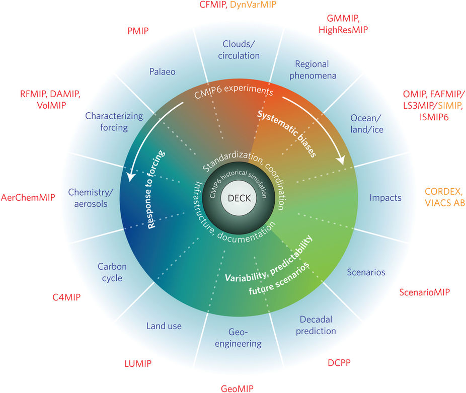
Schematic of the CMIP/CMIP6 experimental design and the 21 CMIP6-Endorsed MIPs. Reproduced with permission from Simpkins (2017).
There is a special issue of the journal Geoscientific Model Development on CMIP6, with 28 published papers covering the overall project and the specific MIPs.
The results of CMIP6 model runs will form the basis of much of the research feeding into the sixth assessment report of the IPCC. However, it is worth noting that CMIP is entirely independent from the IPCC.
How do scientists validate climate models? How do they check them?
Scientists test, or “validate”, their models by comparing them against real-world observations. This might include, for example, comparing the model projections against actual global surface temperatures over the past century.
Climate models can be tested against past changes in the Earth’s climate. These comparisons with the past are called “hindcasts”, as mentioned above.
Scientists do not “tell” their models how the climate has changed in the past – they do not feed in historical temperature readings, for example. Instead, they feed in information on past climate forcings and the models generate a “hindcast” of historical conditions. This can be a useful way to validate models.
Climate model hindcasts of different climate factors including temperature (across the surface, oceans and atmosphere), rain and snow, hurricane formation, sea ice extent and many other climate variables have been used to show that models are able to accurately simulate the Earth’s climate.
There are hindcasts for the historical temperature record (1850-present), over the past 2,000 years using various climate proxies, and even over the past 20,000 years.
Specific events that have a large impact on the climate, such as volcanic eruptions, can also be used to test model performance. The climate responds relatively quickly to volcanic eruptions, so modellers can see if models accurately capture what happens after big eruptions, after waiting only a few years. Studies show models accurately project changes in temperature and in atmospheric water vapour after major volcanic eruptions.
Climate models are also compared against the average state of the climate, known as the “climatology”. For example, researchers check to see if the average temperature of the Earth in winter and summer is similar in the models and reality. They also compare sea ice extent between models and observations, and may choose to use models that do a better job of representing the current amount of sea ice when trying to project future changes.
Experiments where many different models are run with the same greenhouse gas concentrations and other “forcings”, as in model intercomparison projects, provide a way to look at similarities and differences between models.
For many parts of the climate system, the average of all models can be more accurate than most individual models. Researchers have found that forecasts can show better skill, higher reliability and consistency when several independent models are combined.
One way to check if models are reliable is to compare projected future changes against how things turn out in the real world. This can be hard to do with long-term projections, however, because it would take a long time to assess how well current models perform.
Recently, Carbon Brief found that models produced by scientists since the 1970s have generally done a good job of projecting future warming. The video below shows an example of model hindcasts and forecasts compared to actual surface temperatures.
How are climate models “parameterised” and tuned?
As mentioned above, scientists do not have a limitless supply of computing power at their disposal, and so it is necessary for models to divide up the Earth into grid cells to make the calculations more manageable.
This means that at every step of the model through time, it calculates the average climate of each grid cell. However, there are many processes in the climate system and on the Earth’s surface that occur on scales within a single cell.
For example, the height of the land surface will be averaged across a whole grid cell in a model, meaning it potentially overlooks the detail of any physical features such as mountains and valleys. Similarly, clouds can form and dissipate at scales that are much smaller than a grid cell.
To solve this problem, these variables are “parameterised”, meaning their values are defined in the computer code rather than being calculated by the model itself.
The graphic below shows some of the processes that are typically parameterised in models.
Parameterisations may also be used as a simplification where a climate process isn’t well understood. Parameterisations are one of the main sources of uncertainty in climate models.
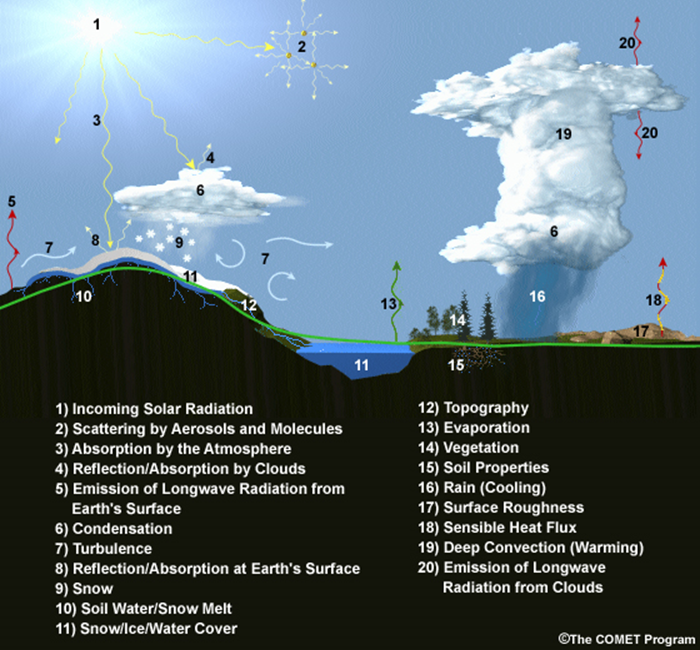
A list of 20 climate processes and properties that typically need to be parameterised within global climate models. Image courtesy of MetEd, The COMET Program, UCAR.
In many cases, it is not possible to narrow down parameterised variables into a single value, so the model needs to include an estimation. Scientists run tests with the model to find the value – or range of values – that allows the model to give the best representation of the climate.
This complex process is known variously as model “tuning” or “calibration”. While it is a necessary part of climate modelling, it is not a process that is specific to it. In 1922, for example, a Royal Society paper on theoretical statistics identified “parameter estimation” as one of three steps in modelling.
Dr James Screen, assistant professor in climate science at the University of Exeter, describes how scientists might tune their model for the albedo (reflectivity) of sea ice. He tells Carbon Brief:
“In a lot of sea ice models, the albedo of sea ice is a parameter that is set to a particular value. We don’t know the ‘correct’ value of the ice albedo. There is some uncertainty range associated with observations of albedo. So whilst developing their models, modelling centres may experiment with slightly different – but plausible – parameter values in an attempt to model some basic features of the sea ice as closely as possible to our best estimates from observations. For example, they might want to make sure the seasonal cycle looks right or there is roughly the right amount of ice on average. This is tuning.”
If all parameters were 100% certain, then this calibration would not be necessary, Screen notes. But scientists’ knowledge of the climate is not perfect, because the evidence they have from observations is incomplete. Therefore, they need to test their parameter values in order to give sensible model output for key variables.
![]()
As most global models will contain parameterisation schemes, virtually all modelling centres undertake model tuning of some kind. A survey in 2014 (pdf) found that, in most cases, modellers tune their models to ensure that the long-term average state of the climate is accurate – including factors such as absolute temperatures, sea ice concentrations, surface albedo and sea ice extent.
The factor most often tuned for – in 70% of cases – is the radiation balance at the top of the atmosphere. This process involved adjusting parameterisations particularly of clouds – microphysics, convection and cloud fraction – but also snow, sea ice albedo and vegetation.
This tuning does not involve simply “fitting” historical observations. Rather, if a reasonable choice of parameters leads to model results that differ dramatically from observed climatology, modellers may decide to use a different one. Similarly, if updates to a model leads to a wide divergence from observations, modellers may look for bugs or other factors that explain the difference.
As NASA Goddard Institute for Space Studies director Dr Gavin Schmidt tells Carbon Brief:
“Global mean trends are monitored for sanity, but not (generally) precisely tuned for. There is a lot of discussion on this point in the community, but everyone is clear this needs to be made more transparent.”
What is bias correction?
While climate models simulate the Earth’s climate well overall – including familiar climatic features, such as storms, monsoon rains, jet streams, trade winds and El Niño cycles – they are not perfect. This is particularly the case at the regional and local scales, where simulations can have substantial deviations from the observed climate, known as “biases”.
These biases occur because models are a simplification of the climate system and the large-scale grid cells that global models use can miss the detail of the local climate.
In these cases, scientists apply “bias correction” techniques to model data, explains Dr Douglas Maraun, head of the Regional Climate Modelling and Analysis research group at the University of Graz, and co-author of a book on “Statistical Downscaling and Bias Correction for Climate Research”. He tells Carbon Brief:
“Imagine you are a water engineer and have to protect a valley against flash floods from a nearby mountain creek. The protection is supposed to last for the next decades, so you have to account for future changes in rainfall over your river catchment. Climate models, even if they resolve the relevant weather systems, may be biased compared to the real world.”
For the water engineer, who runs the climate model output as an input for a flood risk model of the valley, such biases may be crucial, says Maraun:
“Assume a situation where you have freezing temperatures in reality, snow is falling and surface run-off from heavy rainfall is very low. But the model simulates positive temperatures, rainfall and a flash flood.”
In other words, taking the large-scale climate model output as is and running it through a flood model could give a misleading impression of flood risk in that specific valley.
To solve this issue – and produce climate projections that the water engineer can use in designing flood defences – scientist apply “bias correction” to climate model output.
Prof Ed Hawkins, professor of climate science at the University of Reading explains to Carbon Brief:
“Bias correction – sometimes called ‘calibration’ – is the process of accounting for biases in the climate model simulations to provide projections which are more consistent with the available observations.”
Essentially, scientists compare long-term statistics in the model output with observed climate data. Using statistical techniques, they then correct any biases in the model output to make sure it is consistent with current knowledge of the climate system.
Bias correction is often based on average climate information, Maraun notes, though more sophisticated approaches adjust extremes too.
The bias correction step in the modelling process is particularly useful when scientists are considering aspects of the climate where thresholds are important, says Hawkins.
An example comes from a 2016 study, co-authored by Hawkins, on how shipping routes could open through Arctic sea ice because of climate change. He explains:
“The viability of Arctic shipping in future depends on the projected thickness of the sea ice, as different types of ship are unable to travel if the ice reaches a critical thickness at any point along the route. If the climate model simulates too much or too little ice for the present day in a particular location then the projections of ship route viability will also be incorrect.
“However, we are able to use observations of ice thickness to correct the spatial biases in the simulated sea ice thickness across the Arctic and produce projections which are more consistent than without a bias correction.”
In other words, by using bias correction to get the simulated sea ice in the model for the present day right, Hawkins and his colleagues can then have more confidence in their projections for the future.

Russian icebreaker at the North Pole. Credit: Christopher Michel via Flickr.
Typically, bias correction is applied only to model output, but in the past it has also been used within runs of models, explains Maraun:
“Until about a decade ago it was quite common to adjust the fluxes between different model components – for example, the ocean and atmosphere – in every model step towards the observed fields by so-called ‘flux corrections’”.
Recent advances in modelling mean flux corrections are largely no longer necessary. However, some researchers have put forward suggestions that flux corrections could still be used to help eliminate remaining biases in models, says Maraun:
“For instance, most GCMs simulate too cold a North Atlantic, a problem that has knock-on effects, for example, on the atmospheric circulation and rainfall patterns in Europe.”
So by nudging the model to keep its simulations of the North Atlantic Ocean on track (based on observed data), the idea is that this may produce, for example, more accurate simulations of rainfall for Europe.
However, there are potential pitfalls in using flux corrections, he adds:
“The downside of such approaches is that there is an artificial force in the model that pulls the model towards observations and such a force may even dampen the simulated climate change.”
In other words, if a model is not producing enough rainfall in Europe, it might be for reasons other than the North Atlantic, explains Maraun. For example, it might be because the modelled storm tracks are sending rainstorms to the wrong region.
This reinforces that point that scientists need to be careful not to apply bias correction without understanding the underlying reason for the bias, concludes Maraun:
“Climate researchers need to spend much more efforts to understand the origins of model biases, and researchers doing bias correction need to include this information into their research.”
In a recent perspectives article in Nature Climate Change, Maraun and his co-authors argue that “current bias correction methods might improve the applicability of climate simulations” but that they could not – and should not – be used to overcome more significant limitations with climate models.
How accurate are climate model projections of temperature?
One of the most important outputs of climate models is the projection of global surface temperatures.
In order to evaluate how well their models perform, scientists compare observations of the Earth’s climate with models’ future temperatures forecasts and historical temperatures “hindcasts”. Scientists can then assess the accuracy of temperature projections by looking at how individual climate models and the average of all models compare to observed warming.
Historical temperature changes since the late 1800s are driven by a number of factors, including increasing atmospheric greenhouse gas concentrations, aerosols, changes in solar activity, volcanic eruptions, and changes in land use. Natural variability also plays a role over shorter timescales.
If models do a good job of capturing the climate response in the past, researchers can be more confident that they will accurately respond to changes in the same factors in the future.
Carbon Brief has explored how climate models compare to observations in more detail in a recent analysis piece, looking at how surface temperature projections in climate models since the 1970s have matched up to reality.
Model estimates of atmospheric temperatures run a bit warmer than observations, while for ocean heat content models match our best estimate of observed changes quite well.
Comparing models and observations can be a somewhat tricky exercise. The most often used values from climate models are for the temperature of the air just above the surface. However, observed temperature records are a combination of the temperature of the air just above the surface, over land, and the temperature of the surface waters of the ocean.
Comparing global air temperatures from the models to a combination of air temperatures and sea surface temperatures in the observations can create problems. To account for this, researchers have created what they call “blended fields” from climate models, which include sea surface temperatures of the oceans and surface air temperatures over land, in order to match what is actually measured in the observations.
These blended fields from models show slightly less warming than global surface air temperatures, as the air over the ocean warms faster than sea surface temperatures in recent years.
Carbon Brief’s figure below shows both the average of air temperature from all CMIP5 models (dashed black line) and the average of blended fields from all CMIP5 models (solid black line). The grey area shows the uncertainty in the model results, known as the 95% confidence interval. Individual coloured lines represent different observational temperature estimates from groups, such as the Met Office Hadley Centre, NOAA and NASA.
RCP4.5 CMIP5 blended land/ocean model average (in black), two-sigma model range (in grey), and observational temperature records from NASA, NOAA, HadCRUT, Cowtan and Way, and Berkeley Earth from 1970 to 2020. Dashed black line shows original (unblended) CMIP5 multimodel mean. Preliminary value for 2017 is based on temperature anomalies through the end of August. Chart by Carbon Brief using Highcharts.The blended fields from models generally match the warming seen in observations fairly well, while the air temperatures from the models show a bit more warming as they include the temperature of the air over the ocean rather than of the sea surface itself. Observations are all within the 95% confidence interval of model runs, suggesting that models do a good job of reflecting the short-term natural variability driven by El Niño and other factors.
The longer period of model projections from 1880 through 2100 is shown in the figure below. It shows both the longer-term warming since the late 19th century and projections of future warming under a scenario of relatively rapid emissions reductions (called “RCP4.5”), with global temperatures reaching around 2.5C above pre-industrial levels by 2100 (and around 2C above the 1970-2000 baseline shown in the figure).
Same as prior figure, but from 1880 to 2100. Projections through 2100 use RCP4.5. Note that this and the prior graph use a 1970-2000 baseline period. Chart by Carbon Brief using Highcharts.Projections of the climate from the mid-1800s onwards agree fairly well with observations. There are a few periods, such as the early 1900s, where the Earth was a bit cooler than models projected, or the 1940s, where observations were a bit warmer.
Overall, however, the strong correspondence between modelled and observed temperatures increases scientists’ confidence that models are accurately capturing both the factors driving climate change and the level of short-term natural variability in the Earth’s climate.
For the period since 1998, when observations have been a bit lower than model projections, a recent Nature paper explores the reasons why this happened.
The researchers find that some of the difference is resolved by using blended fields from models. They suggest that the remainder of the divergence can be accounted for by a combination of short-term natural variability (mainly in the Pacific Ocean), small volcanoes and lower-than-expected solar output that was not included in models in their post-2005 projections.
Global average surface temperature is only one of many variables included in climate models, and models can be evaluated against many other climate metrics. There are specific “fingerprints” of human warming in the lower atmosphere, for example, that are seen in both models and observations.
Model projections have been checked against temperature observations on the surface, oceans and atmosphere, to historical rain and snow data, to hurricane formation, sea ice extent and many other climate variables.
Models generally do a good job in matching observations globally, though some variables, such as precipitation, are harder to get right on a regional level.
What are the main limitations in climate modelling at the moment?
It is worth reiterating that climate models are not a perfect representation of the Earth’s climate – and nor can they be. As the climate is inherently chaotic, it is impossible to simulate with 100% accuracy, yet models do a pretty good job at getting the climate right.
The accuracy of projections made by models is also dependent on the quality of the forecasts that go into them. For example, scientists do not know if greenhouse gas emissions will fall, and so make estimates based on different scenarios of future socio-economic development. This adds another layer of uncertainty to climate projections.
Similarly, there are aspects of the future that would be so rare in Earth’s history that they’re extremely difficult to make projections for. One example is that ice sheets could destabilise as they melt, accelerating expected global sea level rise.
Yet, despite models becoming increasingly complex and sophisticated, there are still aspects of the climate system that they struggle to capture as well as scientists would like.
Clouds
One of the main limitations of the climate models is how well they represent clouds.
Clouds are a constant thorn in the side of climate scientists. They cover around two-thirds of the Earth at any one time, yet individual clouds can form and disappear within minutes; they can both warm and cool the planet, depending on the type of cloud and the time of day; and scientists have no records of what clouds were like in the distant past, making it harder to ascertain if and how they have changed.
A particular aspect of the difficulties in modelling clouds comes down to convection. This is the process whereby warm air at the Earth’s surface rises through the atmosphere, cools, and then the moisture it contains condenses to form clouds.
On hot days, the air warms quickly, which drives convection. This can bring intense, short-duration rainfall, often accompanied by thunder and lightning.
Convectional rainfall can occur on short timescales and in very specific areas. Global climate models, therefore, have a resolution that is too coarse to capture these rainfall events.
Instead, scientists use “parameterisations” (see above) that represent the average effects of convection over an individual grid cell. This means GCMs do not simulate individual storms and local high rainfall events, explains Dr Lizzie Kendon, senior climate extremes scientist at the Met Office Hadley Centre, to Carbon Brief:
“As a consequence, GCMs are unable to capture precipitation intensities on sub-daily timescales and summertime precipitation extremes. Thus, we would have low confidence in future projections of hourly rainfall or convective extremes from GCMs or coarse resolution RCMs.”
(Carbon Brief will be publishing an article later this week exploring climate model projections of precipitation.)
To help overcome this issue, scientists have been developing very high resolution climate models. These have grid cells that are a few kilometres wide, rather than tens of kilometres. These “convective-permitting” models can simulate larger convective storms without the need of parameterisation.
However, the tradeoff of having greater detail is that the models cannot yet cover the whole globe. Despite the smaller area – and using supercomputers – these models still take a very long time to run, particularly if scientists want to run lots of variations of the model, known as an “ensemble”.
For example, simulations that are part of the Future Climate For Africa IMPALA project (“Improving Model Processes for African Climate”) use convection-permitting models covering all of Africa, but only for one ensemble member, says Kendon. Similarly, the next set of UK Climate Projections, due next year (“UKCP18”), will be run for 10 ensemble members, but for just the UK.
But expanding these convection-permitting models to the global scale is still some way away, notes Kendon:
“It is likely to be many years before we can afford [the computing power for] convection-permitting global climate simulations, especially for multiple ensemble members.”
Double ITCZ
Related to the issue of clouds in global models is that of “double ITCZ”. The Intertropical Convergence Zone, or ITCZ, is a huge belt of low pressure that encircles the Earth near the equator. It governs the annual rainfall patterns of much of the tropics, making it a hugely important feature of the climate for billions of people.
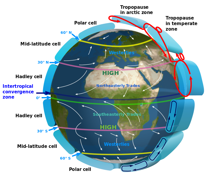
Illustration of the Intertropical Convergence Zone (ITCZ) and the principle global circulation patterns in the Earth’s atmosphere. Source: Creative Commons
The ITCZ wanders north and south across the tropics each year, roughly tracking the position of the sun through the seasons. Global climate models do recreate the ITCZ in their simulations – which emerges as a result of the interaction between the individual physical processes coded in the model. However, as a Journal of Climate paper by scientists at Caltech in the US explains, there are some areas where climate models struggle to represent the position of the ITCZ correctly:
“[O]ver the eastern Pacific, the ITCZ is located north of the equator most of the year, meandering by a few degrees latitude around [the] six [degree line of latitude]. However, for a brief period in spring, it splits into two ITCZs straddling the equator. Current climate models exaggerate this split into two ITCZs, leading to the well-known double-ITCZ bias of the models.”
Most GCMs show some degree of the double ITCZ issue, which causes them to simulate too much rainfall over much of the southern hemisphere tropics and sometimes insufficient rainfall over the equatorial Pacific.
The double ITCZ “is perhaps the most significant and most persistent bias in current climate models”, says Dr Baoqiang Xiang, a principal scientist at the Geophysical Fluid Dynamics Laboratory at the National Oceanic and Atmospheric Administration in the US.
The main implication of this is that modellers have lower confidence in projections for how the ITCZ could change as the climate warms. But there are knock-on impacts as well, Xiang tells Carbon Brief:
“For example, most of current climate models predict a weakened trade wind along with the slowdown of the Walker circulation. The existence of [the] double ITCZ problem may lead to an underestimation of this weakened trade wind.”
(Trade winds are near-constant easterly winds that circle the Earth either side of the equator.)
In addition, a 2015 study in Geophysical Research Letters suggests that because the double ITCZ affects cloud and water vapour feedbacks in models, it therefore plays a role in the climate sensitivity.
![]()
They found that models with a strong double ITCZ have a lower value for equilibrium climate sensitivity (ECS), which indicates that “most models might have underestimated ECS”. If models underestimate ECS, the climate will warm more in response to human-caused emissions than their current projections would suggest.
The causes of the double ITCZ in models are complex, Xiang tells Carbon Brief, and have been the subject of numerous studies. There are likely to be a number of contributing factors, Xiang says, including the way convection is parameterised in models.
For example, a Proceedings of the National Academy of Sciences paper in 2012 suggested that the issue stems from most models not producing enough thick cloud over the “oft-overcast Southern Ocean”, leading to higher-than-usual temperatures over the Southern Hemisphere as a whole, and also a southward shift in tropical rainfall.
As for the question of when scientists might solve this issue, Xiang says it is a tough one to answer:
“From my point of view, I think we may not be able to completely resolve this issue in the coming decade. However, we have made significant progress with the improved understanding of model physics, increased model resolution, and more reliable observations.”
Jet streams
Finally, another common issue in climate models is to do with the position of jet streams in the climate models. Jet streams are meandering rivers of high-speed winds flowing high up in the atmosphere. They can funnel weather systems west to east across the Earth.
As with the ITCZ, climate models recreate jet streams as a result of the fundamental physical equations contained in their code.
However, jet streams often appear to be too “zonal” in models – in other words, they are too strong and too straight, explains Dr Tim Woollings, a lecturer in physical climate science at the University of Oxford and former leader of the joint Met Office-Universities Process Evaluation Group for blocking and storm tracks. He tells Carbon Brief:
“In the real world, the jet veers north a little as it crosses the Atlantic (and a bit the Pacific). Because models underestimate this, the jet is often too far equatorward on average.”
As a result, models do not always get it right on the paths that low-pressure weather patterns take – known as “storm tracks”. Storms are often too sluggish in models, says Woollings, and they do not get strong enough and they peter out too quickly.
There are ways to improve this, says Woollings, but some are more straightforward than others. In general, increasing the resolution of the model can help, Woollings says:
“For example, as we increase resolution, the peaks of the mountains get a little higher and this contributes to deflecting the jets a little north. More complicated things also happen; if we can get better, more active storms in the model, that can have a knock-on effect on the jet stream, which is partly driven by the storms.”
(Mountain peaks get higher as model resolution increases because the greater detail allows the model to “see” more of the mountain as it narrows towards the top.)
Another option is improving how the model represents the physics of the atmosphere in its equations, adds Woollings, using “new, clever schemes [to approximate] the fluid mechanics in the computer code”.
What is the process for improving models?
The process of developing a climate model is a long-term task, which does not end once a model has been published. Most modelling centres will be updating and improving their models on a continuous cycle, with a development process where scientists spend a few years building the next version of their models.
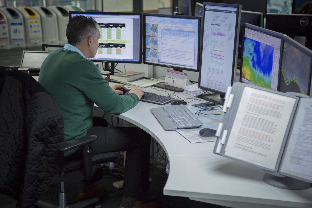
Climate modeller at work in the Met Office, Exeter, UK. Credit: Met Office.
Once ready, the new model version incorporating all the improvements can be released, says Dr Chris Jones from the Met Office Hadley Centre:
“It’s a bit like motor companies build the next model of a particular vehicle so they’ve made the same one for years, but then all of a sudden a new one comes out that they’ve been developing. We do the same with our climate models.”
At the beginning of each cycle, the climate being reproduced by the model is compared to a range of observations to identify the biggest issues, explains Dr Tim Woollings. He tells Carbon Brief:
“Once these are identified, attention usually turns to assessing the physical processes known to affect those areas and attempts are made to improve the representation of these processes [in the model].”
How this is done varies from case to case, says Woollings, but will generally end up with some new improved code:
“This might be whole lines of code, to handle a process in a slightly different way, or it could sometimes just be changing an existing parameter to a better value. This may well be motivated by new research, or the experience of others [modelling centres].”
Sometimes during this process, scientists find that some issues compensate others, he adds:
“For example, Process A was found to be too strong, but this seemed to be compensated by Process B being too weak. In these cases, Process A will generally be fixed, even if it makes the model worse in the short term. Then attention turns to fixing Process B. At the end of the day, the model represents the physics of both processes better and we have a better model overall.”
At the Met Office Hadley Centre, the development process involves multiple teams, or “Process Evaluation Groups”, looking to improve a different element of the model, explains Woollings:
“The Process Evaluation Groups are essentially taskforces which look after certain aspects of the model. They monitor the biases in their area as the model develops, and test new methods to reduce these. These groups meet regularly to discuss their area, and often contain members from the academic community as well as Met Office scientists.
The improvements that each group are working on are then brought together into the new model. Once complete, the model can start to be run in earnest, says Jones:
“At the end of a two- or three-year process, we have a new-generation model that we believe is better than the last one, and then we can start to use that to kind of go back to the scientific questions we’ve looked at before and see if we can answer them better.”
How do scientists produce climate model information for specific regions?
One of the main limitations of global climate models is that the grid cells they are made up of are typically around 100km in longitude and latitude in the mid-latitudes. When you consider that the UK, for example, is only a little over 400km wide, that means it is represented in a GCM by a handful of grid boxes.
Such a coarse resolution means the GCMs miss the geographical features that characterise a particular location. Some island states are so small that a GCM might just consider them as a patch of ocean, notes Prof Michael Taylor, a senior lecturer at the University of the West Indies and a coordinating lead author of the IPCC’s special report on 1.5C. He tells Carbon Brief:
“If you think about the eastern Caribbean islands, a single eastern Caribbean island falls within a grid box, so is represented as water within these global climate models.”
“Even the larger Caribbean islands are represented as one or, at most, two grid boxes – so you get information for just one or two grid boxes – this poses a limitation for the small islands of the Caribbean region and small islands in general. And so you don’t end up with refined, finer scale, sub-country scale information for the small islands.”
Scientists overcome this problem by “downscaling” global climate information to a local or regional scale. In essence, this means taking information provided by a GCM or coarse-scale observations and applying it to specific place or region.

Tobago Cays and Mayreau Island, St. Vincent and The Grenadines. Credit: robertharding/Alamy Stock Photo.
For small island states, this process allows scientists to get useful data for specific islands, or even areas within islands, explains Taylor:
“The whole process of downscaling then is trying to take the information that you can get from the large scale and somehow relate it to the local scale, or the island scale, or even the sub-island scale.”
There are two main categories for methods of downscaling. The first is “dynamical downscaling”. This is essentially running models that are similar to GCMs, but for specific regions. Because these Regional Climate Models (RCMs) cover a smaller area, they can have higher resolution than GCMs and still run in a reasonable time. That said, notes Dr Dann Mitchell, a lecturer in the School of Geographical Sciences at the University of Bristol, RCMs may be slower than their global counterparts:
“An RCM with 25km grid cells covering Europe would take around 5-10 times longer to run than a GCM at ~150 km resolution.”
The UK Climate Projections 2009 (UKCP09), for example, is a set of climate projections specifically for the UK, produced from a regional climate model – the Met Office Hadley Centre’s HadRM3 model.
HadRM3 uses grid cells of 25km by 25km, thus dividing the UK up into 440 squares. This was an improvement over UKCP09’s predecessor (“UKCIP02”), which produced projections at a spatial resolution of 50km. The map below shows how the greater detail that the 25km grid (six maps to the right) affords than the 50km grid (two maps on far left),
RCMs such as HadRM3 can add a better – though still limited – representation of local factors, such as the influence of lakes, mountain ranges and a sea breeze.
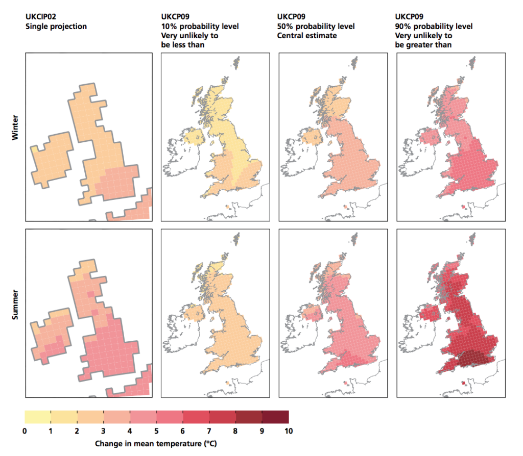
Comparison of changes in seasonal average temperature, winter (top) and summer (bottom), by the 2080s under High Emissions scenarios, from UKCIP02 (far left panels) and as projected for UKCP09 at three probability levels (10, 50 and 90%). Darker red shading shows larger amounts of warming. © UK Climate Projections 2009
Despite RCMs being limited to a specific area, they still need to factor in the wider climate that influences it. Scientists do this by feeding in information from GCMs or observations. Taylor explains how this applies to his research in the Caribbean:
“For dynamical downscaling, you first have to define the domain that you are going to run the model over – in our case, we define a kind of Caribbean/intra-Americas domain – so we limit the modelling to that domain. But, of course, you feed into the boundaries of that domain the output of the large-scale models, so it’s the larger scale model information that drives then the finer-scale model. And that’s the dynamical downscaling – you’re essentially doing the modelling at a finer scale, but over a limited domain, fed in with information at the boundaries.”
It is also possible to “nest”, or embed, RCMs within a GCM, which means scientists can run more than one model at the same time and get multiple levels of output simultaneously.
The second main category of downscaling is “statistical downscaling”. This involves using observed data to establish a statistical relationship between the global and local climate. Using this relationship, scientists then derive local changes based on the large scale projections coming from GCMs or observations.
One example of statistical downscaling is a weather generator. A weather generator produces synthetic timeseries of daily and/or hourly data for a particular location. It uses a combination of observed local weather data and projections of future climate to give an indication of what future weather conditions could be like on short timescales. (Weather generators can also produce timeseries of the weather in the current climate.)
It can be used for planning purposes – for example, in a flood risk assessment to simulate whether existing flood defences will cope with likely future levels of heavy rainfall.
In general, these statistical models can be run quickly, allowing scientists to carry out many simulations in the time it takes to complete a single GCM run.
It is worth noting that downscaled information still depends heavily on the quality of the information that it is based on, such as the observed data or the GCM data feeding in. Downscaling only provides more location-specific data, it does not make up for any uncertainties that stem from the data it relies on.
Statistical downscaling, in particular, is reliant on the observed data used to derive the statistical relationship. Downscaling also assumes that relationships in the current climate will still hold true in a warmer world, notes Mitchell. He tells Carbon Brief:
“[Statistical downscaling] can be fine for well-observed periods of time, or well-observed locations of interest, but, in general, if you push the local system too far, the statistical relationship will break down. For that reason, statistical downscaling is poorly constrained for future climate projections.”
Dynamical downscaling is more robust, says Mitchell, though only if an RCM captures the relevant processes well and the data driving them is reliable:
“Often for climate modelling, the implementation of the weather and climate processes in the dynamical model is not too dissimilar from the coarser global driving model, so the dynamical downscaling only provides limited improvability of the data. However, if done well, dynamical downscaling can be useful for localised understanding of weather and climate, but it requires a tremendous amount of model validation and in some cases model development to represent processes that can be captured at the new finer scales.”
Updated on 15 January 2018 to clarify that the one million dollar prize for solving the N-S equations are for proving the existence of a solution in all circumstances, and that the grid boxes only converge towards the poles when the grid is based on latitude and longitude.
Carbon Brief would like to thank all the scientists who helped with the preparation of this article.
Tomorrow: An interactive timeline of the key developments in climate modelling over the past century.
-
Q&A: How do climate models work?
-
Everything you ever needed to know about climate models